Quick Voltage Dip Calculator for Generators: Estimate Step-Load Drops from Alternator Inputs

Quick voltage dip estimation speeds generator sizing and transient response analysis for operational reliability planning.

This calculator predicts step load-induced voltage sags using alternator reactances and rotor inertia data accurately.

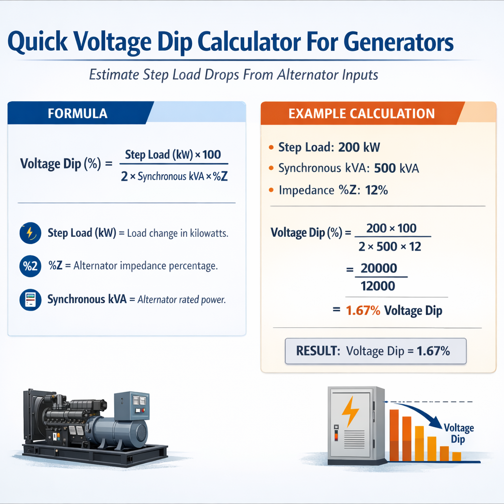
Quick Voltage Dip Estimator for Generators (Step Load from Alternator Short-Circuit Data)

Generator rated apparent power (kVA)

Step load active power (kW)

Step load power factor (–)

Subtransient reactance Xd'' (p.u.)

Advanced options

Rated line-to-line voltage (V)

System frequency (Hz) 50 Hz (IEC regions) 60 Hz (NEMA regions) Other / special frequency

Initial total active load before step (kW)

Initial average power factor (–)

AVR transient support factor (% of dip corrected) 0% (no fast AVR correction, worst case) 20% (basic AVR response) 40% (standard AVR response) 60% (strong AVR response) Custom value

Custom AVR support factor (%)

Upload a generator nameplate or single-line diagram photo to suggest reasonable input values.

📷 Fill inputs from AI photo

⚡ More electrical calculators Reiniciar Copiar Compartir

Enter generator rating, step load and subtransient reactance to estimate the voltage dip.

🧠 Explicar mi resultado 🔍 Revisar mis datos

Calculation method (simplified generator step-load voltage dip):

• Rated apparent power: S_rated [kVA]
• Step active power: P_step [kW]
• Step power factor: cos φ_step (dimensionless)
• Step apparent power: S_step [kVA]
• Subtransient reactance: Xd'' (per-unit)
• AVR transient support factor: F_AVR [% of dip corrected]

1) Step apparent power:

S_step [kVA] = P_step [kW] / cos φ_step

2) Alternator subtransient short-circuit power:

S_k'' [kVA] = S_rated [kVA] / Xd''

3) Theoretical per-unit voltage dip caused by the step:

ΔV_pu ≈ S_step / S_k'' = S_step × Xd'' / S_rated

4) Theoretical voltage dip in percent:

ΔV_theoretical [%] = 100 × S_step × Xd'' / S_rated

5) Effective voltage dip with AVR support:

ΔV_effective [%] = ΔV_theoretical × (1 − F_AVR / 100)

If rated voltage is given (V_rated), the estimated minimum line-to-line voltage is:

V_min [V] ≈ V_rated × (1 − ΔV_effective / 100)

The initial and final loading levels are estimated using the initial kW and power factor (if provided):

S_initial [kVA] ≈ P_initial [kW] / cos φ_initial
S_final [kVA] ≈ S_initial + S_step
Loading before step [%] ≈ 100 × S_initial / S_rated
Loading after step [%] ≈ 100 × S_final / S_rated

Generator size (kVA)	Typical Xd'' (p.u.)	Recommended single step voltage dip limit (%)
50 – 250	0.20 – 0.30	10 – 15% for normal loads, up to 20% for motor starting
250 – 1000	0.15 – 0.25	10 – 15% for most installations
1000 – 2500	0.12 – 0.20	8 – 12% for sensitive loads, 15% maximum
> 2500	0.10 – 0.18	5 – 10% where stringent voltage quality is

Technical frequently asked questions

How accurate is this quick voltage dip estimation?

This calculator uses a standard subtransient short-circuit power approach, assuming that the voltage dip is dominated by the alternator subtransient reactance and that the AVR response is represented by a single correction factor. For typical three-phase generators with conventional AVRs, the estimate is usually within a few percentage points of detailed transient simulations, provided that Xd'' is accurate and the step power factor is realistic.

Which value of Xd'' should I use if the datasheet gives several reactances?

Use the direct-axis subtransient reactance Xd'' in per-unit on the generator’s own base (rated kVA and rated voltage). Do not use transient or synchronous reactances. If Xd'' varies with connection or excitation system, select the value specified for the alternator configuration used in your generator set.

Does the existing load level before the step change the voltage dip?

For a first-order estimate based on subtransient short-circuit power, the voltage dip mainly depends on the incremental step apparent power relative to the alternator rating and Xd''. The initial loading has only a second-order influence, so it is reported for context but does not modify the simplified dip formula here. For highly loaded sets or very sensitive installations, a full transient stability study is recommended.

How should I choose the AVR transient support factor?

If you have manufacturer test curves, you can infer how much of the initial dip is corrected within the first few cycles and enter that as the AVR support factor. Otherwise, 20–40% is a reasonable engineering assumption for modern digital AVRs, while 0–20% is more typical for basic or poorly tuned regulators.

Fundamental model, scope and practical assumptions for a fast calculator

A pragmatic quick calculator models a synchronous alternator as an internal electromotive force (E) behind a series reactance that changes with time: subtransient Xd'', transient Xd', and steady-state Xd. The immediate terminal voltage response to a step increase in load is dominated by Xd''; thereafter the generator voltage recovers toward the Xd' response as damper windings and flux decay act with characteristic time constants. For a fast, conservative estimate we assume nominal pre-event terminal voltage V_nom = 1.0 pu and use the generator rated MVA as the per-unit base. Key simplifications used:

• Balanced three-phase step loads (useful for motor starting and balanced block loading).
• Generator pre-fault terminal voltage magnitude V_pre = 1.0 pu and internal emf E ≈ 1.0 pu (adjustable for AVR setpoint).
• Immediate voltage dip computed using subtransient reactance Xd''; intermediate values use Xd'.
• Power factor of the step load is specified; reactive component computed accordingly.

Core equations and phasor method for voltage dip estimation

All formulas are expressed in per-unit on the generator MVA and nominal terminal voltage base. Typical notation: P is active power (MW), Q is reactive power (MVAr), S = P + jQ (MVA). Use S_base = generator rated MVA and V_base = rated line-line voltage.

Compute complex per-unit step apparent power:

Model the generator internal voltage (behind reactance X) as E_pu (assumed ~1.0) and compute new terminal voltage phasor for the immediate response (use X = Xd''):

Voltage dip magnitude (per-unit) referenced to pre-event 1.0 pu is:

Expressed as percent:

Notes on signs and conjugation:

• Complex power S = P + jQ = V * I_conj. Therefore I_conj = S / V and I = conjugate(S / V).
• If V_pre = 1.0∠0, then I_pu angle equals -atan2(DeltaQ, DeltaP) (current lags for inductive loads).
• Multiplication by j rotates phasors by +90° (j*I) and -j rotates by -90° (−j*I). The expression E − jX I accounts for the voltage drop across reactance.

Phasor arithmetic explicit expansion

For clarity, expand I_pu magnitude and angle: Convert current to rectangular components: Then compute V_drop = j * Xd'' * I_pu = j * Xd'' * (I_real + j*I_imag) = j*Xd''*I_real + j^2 * Xd''*I_imag = j*Xd''*I_real - Xd''*I_imag. Finally:

V_new_real = E_real - V_drop_real = E_pu - ( - Xd'' * I_imag ) = E_pu + Xd'' * I_imag

Then magnitude: All steps are implemented in the quick calculator to yield a numerical percent voltage dip.

Variable definitions, units and typical values

• DeltaP: step change in active power, MW (positive for load increase).
• DeltaQ: step change in reactive power, MVAr (positive for inductive load).
• S_base: generator rated apparent power, MVA.
• V_pu: terminal voltage pre-event, per-unit (nominally 1.0).
• E_pu: internal emf per-unit, typical 0.98–1.05 depending on AVR.
• Xd'': subtransient reactance, per-unit (for immediate response).
• Xd': transient reactance, per-unit (intermediate recovery).
• Xd: synchronous reactance, per-unit (steady-state).
• Td'': subtransient decay time (s), Td': transient decay time (s).
• H: inertia constant (s) - stored energy at rated speed per MVA rating.

Below is a table with typical ranges for synchronous generator parameters across common sizes.

Step-by-step algorithm implemented in the quick calculator

1. User inputs: Generator rating S_base (MVA), nominal voltage V_nom (kV), E_pu, Xd'', Xd', Xd, DeltaP (MW) and load power factor (pf) or DeltaQ (MVAr). Also choose the time after step for selecting Xd'' (immediate), Xd' (after subtransient decay), or Xd (steady-state).
2. Compute DeltaQ if pf provided:

   DeltaQ = DeltaP * tan(acos(pf)) for lagging (inductive) loads; sign convention: inductive positive.

3. Compute complex DeltaS_pu = (DeltaP + j*DeltaQ) / S_base.
4. Compute I_pu = conjugate(DeltaS_pu) / V_pu (with V_pu assumed 1.0 unless the user provides a different pre-event voltage).
5. Select reactance X = Xd'' or Xd' depending on chosen time window.
6. Compute V_new_pu = E_pu - j * X * I_pu and its magnitude.
7. Compute Vdip_percent = (1.0 - |V_new_pu|) * 100 and flag if it exceeds user-defined thresholds (e.g., 5%, 10%).

Practical effects, AVR and governor interaction, and time evolution

While the immediate dip is dominated by Xd'', the subsequent recovery and steady-state voltage are affected by:

• Excitation control: Automatic Voltage Regulator (AVR) increases field current and internal emf E over the AVR response time; this reduces steady-state dip but only after a control time constant.
• Prime mover and governor response: changes active power supply, affecting rotor angle and may induce frequency deviations for large steps.
• Inertia H: determines the rate of change of rotor speed and thus frequency deviation; low H leads to faster frequency changes which can interact with voltage behavior via flux linkage.

A more accurate transient simulation solves the machine differential equations and AVR/governor control loops. The quick calculator provides conservative, fast estimates useful for sizing and planning.

Table: conversion and quick reference constants

Example case 1 — Small industrial generator starting a motor (complete worked solution)

Scenario:

• Generator: S_base = 0.5 MVA (500 kVA), V_nom = 400 V (LV), E_pu = 1.0
• Machine parameters: Xd'' = 0.22 pu, Xd' = 0.30 pu
• Load step: motor starting presenting step apparent power DeltaP_start = 200 kW with starting power factor estimated 0.3 lagging (typical heavy motor inrush)
• Time of interest: immediate (use Xd'')

Step calculations: 1) Compute DeltaQ from pf: Numerical: 2) Complex DeltaS (MW/MVAr): 3) Per-unit DeltaS_pu: 4) Compute I_pu (assuming V_pu = 1.0 and using conjugate): 5) Use X = Xd'' = 0.22 pu and compute j*X*I_pu:

j * X * I_pu = j * 0.22 * (0.400 - j1.282) = j*0.088 - j^2 * 0.282 = j0.088 + 0.282 → equals 0.282 + j0.088

6) Terminal voltage phasor V_new_pu = E_pu - jX I_pu = 1.0 - (0.282 + j0.088) = 0.718 - j0.088 7) Magnitude: 8) Voltage dip: Interpretation:

• A 27.7% sag is severe and will likely trip sensitive loads or fail to start the motor properly. This matches expectations for an LV generator with heavy motor inrush.
• Mitigation: use soft-start, pre-insertion resistors, or staged starting; consider larger genset or motor start sequencing.

Example case 2 — Medium-sized plant generator sudden resistive block load

Scenario:

• Generator: S_base = 5.0 MVA, V_nom = 11 kV, E_pu = 1.02 (AVR holding slightly above unity)
• Machine parameters: Xd'' = 0.15 pu, Xd' = 0.22 pu
• Load step: DeltaP = 2.0 MW applied instantaneously, PF = 0.95 (nearly resistive)
• Time horizon: immediate (Xd'') and intermediate (Xd')

Step calculations — immediate: 1) Compute DeltaQ: 2) DeltaS: 3) DeltaS_pu: 4) I_pu = conjugate(DeltaS_pu) = 0.400 - j0.1316 pu 5) j * Xd'' * I_pu: 6) V_new_pu = E_pu - (0.0197 + j0.06) = 1.02 - 0.0197 - j0.06 = 1.0003 - j0.06 7) Magnitude: 8) Voltage dip: Interpretation immediate:

• The computed value shows no sag; in fact the terminal voltage is slightly above 1.0 pu because E_pu was 1.02 — an AVR-maintained excitation kept voltage tightly regulated for a nearly resistive load.
• In practice the AVR cannot react instantaneously; if E_pu were 1.0 pre-event the initial dip would be small but nonzero. Using E_pu = 1.0 yields a dip of about 1.97% (compute separately with E=1.0 if needed).

Intermediate (after subtransient decay → use Xd'): Repeat step with Xd' = 0.22 pu: Interpretation:

• After the very fast subtransient effect decays, the generator exhibits a small dip ~0.5% which the AVR can correct over its regulation time. This is acceptable for most industrial equipment.

These two worked examples demonstrate how generator size, reactance and load power factor determine the severity of the voltage dip.

Design thresholds, standards and measurement practices

Voltage dips are covered by several international standards and grid codes. Relevant references:

• IEC 61000-4-11 — Electromagnetic compatibility (EMC) — tests and measurement techniques for voltage dips, short interruptions and voltage variations immunity tests. https://www.iec.ch
• EN 50160 — Voltage characteristics of electricity supplied by public distribution systems (defines tolerances and limits). https://www.en-standard.eu
• IEC 60034 series — rotating machinery characteristics and testing (machine reactance and time-constant measurement). https://www.iec.ch
• ISO 8528 — Reciprocating internal combustion engine driven alternating current generating sets — provides guidance on testing and performance. https://www.iso.org
• IEEE references: IEEE Std 421.5 (excitation system models) and IEEE Std C37.x family for generator protection and testing procedures. https://www.ieee.org

Measurement recommendations:

1. Use a transient recorder or power quality analyzer sampling at ≥ 2 kS/s per phase for accurate capture of step events and sub-cycle behaviour.
2. Record pre-event steady-state voltage and speed; log AVR and governor control outputs if available.
3. Apply synchronization: correlate event time with protection/log events and load switching timestamps.
4. Perform factory or field short-circuit and reactance tests to obtain accurate Xd'', Xd' and time constants rather than relying solely on catalog values.

Mitigation methods and practical recommendations

If the quick calculator predicts unacceptable dips, use these mitigations:

• Load sequencing: stagger the application of large motors or resistive loads.
• Soft-start devices for motors (VFDs, reduced voltage starters) to limit starting current.
• Limit inrush: pre-insertion resistors or controlled tap changers.
• Increase generator sizing or add spinning reserve (larger inertia H reduces frequency excursions).
• AVR tuning: faster excitation response reduces steady-state sag, but beware of instability if too aggressive.
• Energy storage (batteries, supercapacitors) or dynamic reactive power compensators (STATCOM) for very fast sag support.

Implementation notes for an online quick voltage dip calculator

To implement a robust calculator:

• Allow user input of DeltaP and either pf or DeltaQ; provide sensible defaults for Xd'', Xd' and E_pu based on generator class.
• Offer time-slice selection: immediate (Xd''), intermediate (Xd'), steady-state (Xd).
• Compute phasors with complex arithmetic and provide both per-unit and absolute voltage outputs (Vrms in nominal volts).
• Include warnings if computed current exceeds generator thermal or protection limits.
• Provide suggested mitigations and flags when dips exceed thresholds (e.g., 10% or 20% depending on site requirements).
• Document normative references and measurement steps to validate calculated estimates.

Limitations and when to use full dynamic simulation

The quick calculator provides a valuable engineering estimate but is limited:

• For unbalanced faults, negative- and zero-sequence reactances and asymmetrical current components must be modeled (not covered in the basic model).
• If AVR or governor control interactions critically affect voltage, a multi-machine dynamic simulation (EMT or phasor time-domain) is required.
• Breaker operating times, network impedance external to generator, and transformer tap-changers require network-level modeling.

When to escalate:

1. Large systems with multiple generators synchronised and significant network impedance.
2. Events that trigger protection actions or where protection settings must be coordinated.
3. Detailed mitigation design involving STATCOMs, synchronous condensers, or firmware control tuning.

Summary of best practice checks before relying on quick-calculator outputs

• Verify generator parameters (Xd'', Xd', Xd, Td'', Td') with manufacturer test data.
• Confirm S_base and V_base choices; ensure per-unit bases are consistent.
• Check pre-event E_pu setting and AVR time constants; instrument if necessary.
• Use the calculator for screening and early design; follow up with transient simulation for critical cases.

Authoritative references and further reading

• IEC 61000-4-11 — Voltage dips, short interruptions and voltage variations immunity tests: https://www.iec.ch/
• EN 50160 — Voltage characteristics of public distribution networks: https://www.en-standard.eu/
• ISO 8528 series for generator set performance: https://www.iso.org/standard/
• IEEE Std 421.5 — Recommended practice for excitation system models for power system stability studies: https://standards.ieee.org/
• Manufacturer technical papers on generator transient reactance and testing (Siemens, ABB, GE) — consult vendor machine datasheets for accurate Xd'' and time constants.

Use this quick voltage dip methodology as a screening and planning tool. For final design or protection coordination, complement these results with manufacturer data and dedicated transient stability or EMT simulations.