This guide explains converting connected load to demand load with precise engineering calculations and factors.
Step-by-step methods include diversified demand factors, diversity application, and aggregated total computations for design verificationConvert Connected Load to Demand Load — Step-by-Step (Demand Factor & Diversified Total)
Scope and normative references
This technical article provides a detailed engineering method to convert connected load into demand load, calculate demand factors, and compute diversified totals for building electrical systems. It is intended for electrical engineers, designers, and technical reviewers involved in load estimation, feeder and service sizing, and energy management.
Primary standards and guidance
- NFPA 70 (National Electrical Code) — service and feeder demand calculations: https://www.nfpa.org/
- IEC 60364 series — requirements for electrical installations: https://www.iec.ch/
- CIBSE Guides — non-domestic building diversity and internal gains: https://www.cibse.org/
- IET Wiring Regulations (BS 7671) — UK practice and demand factors: https://www.theiet.org/
- IEEE Std. 141 (Red Book) — system design fundamentals and practical engineering: https://ieeexplore.ieee.org/
Fundamental definitions and relationships
Connected load (Qc)
The connected load (Qc) is the sum of the nameplate ratings or declared maximum demands of all electrical equipment expected to be installed, expressed in watts (W) or volt-amperes (VA).
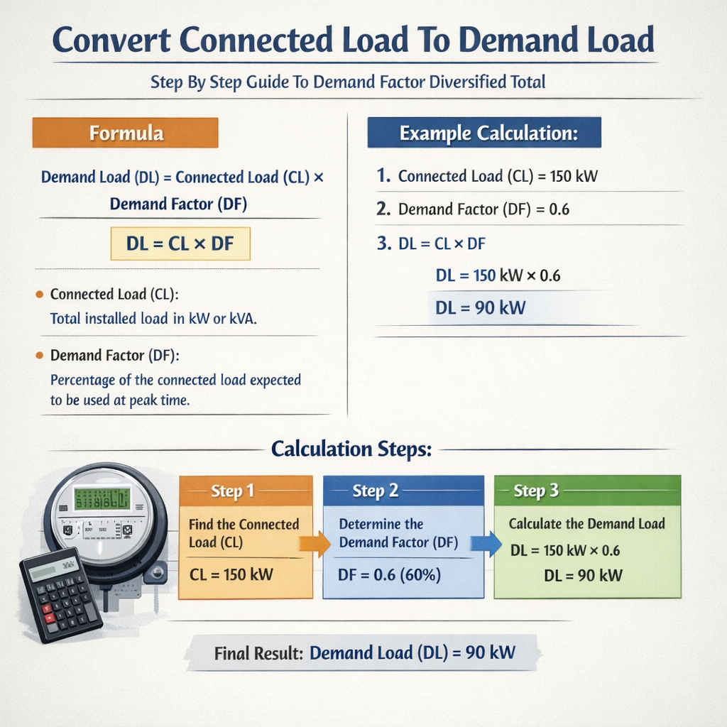
Demand load (Qd) and demand factor (DF)
Demand load (Qd) is the actual maximum power expected to be drawn simultaneously by the installation during normal operation. The demand factor (DF) relates Qd to Qc.
Basic formula:
- Qd — Demand load (W or VA)
- Qc — Connected load (W or VA)
- DF — Demand factor (dimensionless, 0–1)
Diversity factor (μ)
Diversity factor (μ) is defined as the ratio of the sum of individual maximum demands to the maximum observed combined demand:
Note: Diversity factor ≥ 1. When applied to groups it reduces the calculated sizing by accounting for non-coincidence of loads.
Methodology: Step-by-step conversion from connected to demand load
- Inventory all connected loads, specifying categories (lighting, receptacles, HVAC, motors, specialty equipment) and units (W or VA).
- Group loads into logical diversity groups based on usage patterns (e.g., lighting, HVAC, appliances, motors).
- Assign appropriate demand factors for each group using normative tables, manufacturer data, measured diversity, or engineering judgment.
- Convert single-phase and motor nameplate data to consistent units (VA when using apparent power).
- Apply group demand factors and sum the resulting demanded powers to obtain Qd_total.
- Verify peak diversity: assess simultaneity of loads and adjust DF or apply diversity factors between groups as required.
- Apply power factor correction or consider worst-case power factor for conductor and transformer sizing if calculating apparent power (VA).
Notes on grouping
- Group by function and expected simultaneity (e.g., residential cooking vs. lighting vs. HVAC).
- Separate continuous loads (operating for more than three hours) since codes may require continuous load treatment (e.g., +125% for conductor sizing per some jurisdictions).
- Identify standby and emergency loads that have different diversity and reliability requirements.
Typical demand factor values and diversity tables
Below are engineering-typical values commonly used for preliminary design. These are not replacements for code-specific tables, but provide engineering starting points.
| Load Category | Typical Connected Load Characteristics | Recommended Demand Factor (DF) | Notes and Typical Range |
|---|---|---|---|
| Residential lighting | Interior + exterior lighting | 0.6 – 0.9 | Lower DF for larger multi-unit buildings; 0.6–0.8 common for apartments |
| Residential small appliances & general-use receptacles | Kitchen circuits, laundry, general outlets | 0.4 – 0.6 | NEC provides specific allowances per dwelling unit; use conservative values for feeders |
| Electric ranges / cooking equipment | High-power, low-coincidence appliances | 0.75 – 1.0 (per unit) / 0.5–0.8 (group diversity) | Often treated with individual allowances or demand tables |
| Commercial lighting | Offices, retail | 0.6 – 0.9 | DF depends on occupancy sensors and schedule diversity |
| HVAC (central plant) | Large chillers, AHUs, rooftop units | 0.6 – 1.0 | Consider diversity between units; simultaneous operation may be unlikely |
| Motors (industrial) | Pumps, compressors, motors | 0.5 – 1.0 depending on simultaneity | Large motors often considered at full load; smaller motors grouped with diversity 0.6–0.8 |
| Elevators | Traction and hydraulic | 0.3 – 0.8 | High diversity due to infrequent simultaneous use |
| Special loads (medical, data centers) | Critical loads with high availability | 0.9 – 1.0 | Use conservative factors; separate redundancy considerations |
| Connected Load Range (Lighting) | Suggested Demand Factor (Lighting) | Rationale |
|---|---|---|
| Up to 10 kW | 0.9 | Small installations with high coincidence |
| 10–50 kW | 0.7 – 0.85 | Moderate diversity; occupancy pattern variations |
| 50–200 kW | 0.6 – 0.75 | Greater chance of non-coincidence; zoning reduces simultaneity |
| >200 kW | 0.6 | Large complexes show significant diversity due to distribution of spaces |
Mathematical formulations and variable explanations
Below are formulas used for converting connected load to demand load and computing diversified totals. Variables include power (P), apparent power (S), power factor (pf), and group demand factors (DF).
Single-group demand
Equation:
- Qd_group — Demand for the specific group (W or VA)
- Qc_group — Connected load of the group (W or VA)
- DF_group — Demand factor for the group (0–1)
Combined diversified total for multiple groups
Equation:
- Qc_i — Connected load of group i
- DF_i — Demand factor for group i
- Σ — Summation over all load groups
Diversity interaction between groups (non-coincidence)
When groups have low simultaneity, apply an additional diversity multiplier or explicitly model simultaneity using probabilistic or time-of-use data:
- S_i — Simultaneity factor for group i (0–1), where S_i < 1 reduces demand based on expected non-coincidence
Apparent power and power factor
For equipment rated in watts (real power) but sizing transformers and conductors requires apparent power (VA):
- S — Apparent power (VA)
- P — Real power (W)
- pf — Power factor (0–1)
Use conservative pf values when uncertain (e.g., 0.8 lagging) or use measured pf provided by equipment manufacturers.
Worked Example 1 — Multi-family residential feeder sizing
Scenario: A three-floor apartment building with six identical units per floor. Each apartment contains the following nameplate connected loads:
- Lighting: 1.2 kW
- General-use receptacles (appliances, outlets): 2.4 kW
- Electric range: 6.0 kW
- Electric water heater (storage): 4.5 kW (controlled water heating schedule)
- Space heating (heat pump, rated): 3.0 kW
Compute total connected load and estimated demand load for feeder design using engineering demand factors from the tables.
Step 1 — Sum connected loads per apartment
Step 2 — Connected load for entire building
Step 3 — Assign group demand factors
- Lighting DF_light = 0.7 (multi-unit building)
- General receptacles DF_recept = 0.5
- Ranges DF_range_group = 0.6 (group diversity for multiple ranges)
- Water heaters DF_wh = 0.4 (diversified due to storage and timer)
- Space heating DF_heat = 0.9 (high coincidence in cold weather)
Step 4 — Compute demanded loads per group for building
Compute total connected per group:
- Qc_light_total = 18 × 1.2 = 21.6 kW
- Qc_recept_total = 18 × 2.4 = 43.2 kW
- Qc_range_total = 18 × 6.0 = 108.0 kW
- Qc_wh_total = 18 × 4.5 = 81.0 kW
- Qc_heat_total = 18 × 3.0 = 54.0 kW
Apply demand factors:
- Qd_light = 21.6 × 0.7 = 15.12 kW
- Qd_recept = 43.2 × 0.5 = 21.6 kW
- Qd_range = 108.0 × 0.6 = 64.8 kW
- Qd_wh = 81.0 × 0.4 = 32.4 kW
- Qd_heat = 54.0 × 0.9 = 48.6 kW
Step 5 — Sum demanded loads
Step 6 — Apply simultaneity adjustment if applicable
If maintenance records show non-coincidence between ranges and heating (e.g., cooking peaks during evening and heating peaks in morning), assume a simultaneity factor S_range = 0.85 and S_heat = 0.9. Recompute adjusted:
Step 7 — Convert to apparent power for transformer sizing (pf = 0.9 assumed)
Result: Use standard transformer rating ≥ 200 kVA to provide margin. Verify continuous load provisions and local code multipliers (e.g., conductor ampacity 125% for continuous).
Worked Example 2 — Commercial office building with diverse systems
Scenario: A medium office building with the following connected loads on a floor:
- Lighting: 40 kW
- General receptacles (IT + office equipment): 60 kW
- Cooling (DX HVAC units): 120 kW
- UPS (critical loads): 30 kW
- Elevator bank: 20 kW
Step 1 — Assign demand factors
- Lighting DF_light = 0.65
- Receptacles DF_recept = 0.6 (diversity for office equipment)
- Cooling DF_HVAC = 0.85 (multiple units with partial simultaneous operation)
- UPS DF_ups = 1.0 (critical loads considered fully demanded for sizing backup capacity)
- Elevators DF_elev = 0.35 (low simultaneous peak)
Step 2 — Apply demand factors
- Qd_light = 40 × 0.65 = 26.0 kW
- Qd_recept = 60 × 0.6 = 36.0 kW
- Qd_HVAC = 120 × 0.85 = 102.0 kW
- Qd_UPS = 30 × 1.0 = 30.0 kW
- Qd_elev = 20 × 0.35 = 7.0 kW
Step 3 — Grouped diversified total
Step 4 — System-level adjustments and transformer sizing
If this is a 5-floor building with similar loads per floor but HVAC centrally distributed, assume floor diversity for lighting and receptacles (S_floor = 0.9). For UPS and central HVAC assume near full coincidence for critical design.
Total floor-connected loads (5 floors): Qc_total = 5 × (40 + 60 + 120 + 30 + 20) = 5 × 270 = 1350 kW connected.
Assume central HVAC is not strictly five times; use central diversity DF_central_HVAC = 0.95 for central plant: Qd_HVAC_total = 120 × 5 × 0.95 = 570 kW
Step 5 — Apparent power and transformer selection (pf = 0.92)
Select transformer(s) to meet total with redundancy (e.g., two 800 kVA paralleled or a single 1,250 kVA with standby).
Practical guidance, measurement and verification
- Where possible, use measured load profiles (interval metering) to derive realistic demand and simultaneity statistics rather than solely nameplate-based DF.
- For critical systems (medical, data centers), adhere to stricter design practice where DF is near 1.0 and additional reliability is required.
- Document assumptions for DF, simultaneity factors, and continuous-load adjustments; present sensitivity analyses for different DF scenarios.
- When calculating conductor ampacity and protective device ratings, apply code-required multipliers for continuous loads (e.g., 125% in many codes) and equipment temperature ratings.
Advanced methods: probabilistic and time-of-use modelling
For large or complex installations consider probabilistic methods (Monte Carlo simulation) or time-of-use stacking to model the likelihood of coincident peaks. These techniques require:
- Load probability distributions for each group (based on historical or measured data).
- Statistical correlation coefficients between groups (coincidence indexes).
- Simulation runs to compute percentile peaks (e.g., 95th percentile demand).
Probabilistic approaches often yield more economical infrastructure sizing while controlling reliability risk to acceptable levels.
Verification against codes and safety factors
- Always cross-check engineering DF with code-prescribed demand tables where applicable (e.g., NEC load calculation articles).
- Include additional margins for future expansion and measurement uncertainty (commonly 10–20% contingency for early-stage design).
- For emergency and standby design, follow NFPA 110, NEC Article 700–701, and local jurisdictional rules.
Common pitfalls and mitigation
- Over-reliance on nameplate ratings without usage pattern analysis — mitigate by metering representative loads.
- Misapplication of demand factors across incompatible load groups — mitigate by proper grouping and discipline-specific DF selection.
- Ignoring harmonic effects and power quality — check non-linear loads and derate transformers/conductors accordingly.
- Neglecting simultaneous start-up currents for motor-dominant systems — conduct motor starting study or apply diversity conservatively for starters.
Tables for engineers: motor diversity and starting considerations
| Motor Type | Typical Nameplate (% of connected) | Diversity Factor (for grouped small motors) | Starting Current Estimate (Inrush) |
|---|---|---|---|
| Large fixed-speed motor (>50 kW) | 100% | 0.9 – 1.0 | 5–8 × full load current |
| Small motors (<5 kW) | 100% | 0.5 – 0.8 | 3–6 × full load current |
| Multiple pump bank | Sum of nameplates | 0.6 – 0.85 (depends on duty) | Varies — assume worst-case starting one at a time |
Documentation and reporting checklist
- Complete inventory of connected loads and basis of values (manufacturer datasheets, nameplates).
- Grouping rationale and assigned demand factors with citations to standards or measured data.
- Step-by-step calculations for Qc, Qd per group, and aggregated diversified totals.
- Assumptions on power factor, simultaneity, and continuous load treatment.
- Recommendations for transformer sizing, conductor ampacity, and protective device settings.
- Sensitivity analysis showing effect of ±10–20% change in DF on equipment sizing.
References and further reading
- National Fire Protection Association (NFPA) — NFPA 70: National Electrical Code. https://www.nfpa.org/
- International Electrotechnical Commission — IEC 60364 series overview. https://www.iec.ch/
- CIBSE — Guides on building services and diversity factors. https://www.cibse.org/
- IET — Wiring Regulations (BS 7671) guidance. https://www.theiet.org/
- IEEE — Power engineering guides and standards. https://ieeexplore.ieee.org/
- IEC/IEEE documents on power quality for non-linear loads and harmonics.
Final recommendations for practitioners
- Start with conservative demand factors for critical infrastructure and refine with measured data during commissioning.
- Document and justify every DF and simultaneity assumption to facilitate future inspections and upgrades.
- Use probabilistic methods for complex systems where preliminary deterministic DFs produce marginal sizing outcomes.
- Always cross-reference your engineering solution with local code requirements and the latest editions of referenced standards.
Accurate conversion from connected load to demand load requires disciplined grouping, normative references, and iterative verification. Use the tables, formulas, and worked examples above as a practical engineering framework for robust feeder, transformer, and service design.