Electrical Resistivity Unit Converter: Convert Ohmmeter Readings to ohm-cm for Grounding

This article provides technical guidance for converting ohmmeter readings to ohm-centimeter units for grounding systems.

Procedures, formulas, normative references, and examples ensure accurate resistivity conversion and practical grounding assessments methods.

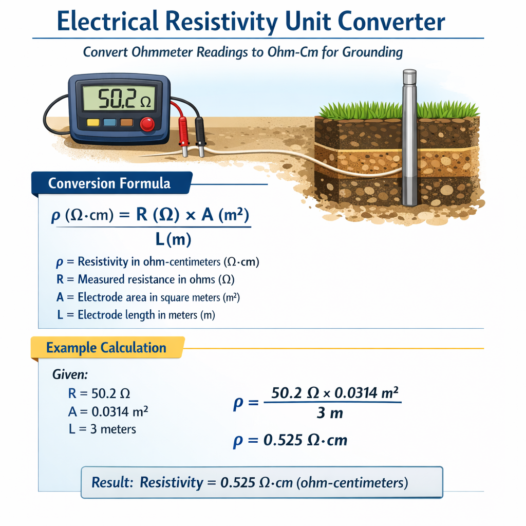
Soil Electrical Resistivity Unit Converter (Ohm·m to Ohm·cm for Grounding Design)

Measured soil resistivity value

Input unit Ohm·meter (Ω·m) – common tester output Ohm·centimeter (Ω·cm) kiloohm·centimeter (kΩ·cm)

Target unit for conversion Ohm·centimeter (Ω·cm) – typical for grounding references Ohm·meter (Ω·m) kiloohm·centimeter (kΩ·cm)

Advanced options

Soil type (qualitative) Custom / not specified Very moist clay / peat Loam / agricultural soil Dry sand / gravel Rocky / bedrock

Reference soil temperature (°C)

Electrode spacing (m)

Technical notes

Upload a clear photo of the instrument display, nameplate, or test diagram to suggest suitable input values.

📷 Rellene datos con foto IA

⚡ More electrical calculators Reiniciar Copiar Compartir

Enter a soil resistivity value to obtain the converted unit.

🧠 Explicar mi resultado 🔍 Revisar mis datos

Formulas used for resistivity unit conversion

The calculator assumes a linear relationship between resistivity units based on length conversion:

• Basic length relationship: 1 meter (m) = 100 centimeters (cm).
• Resistivity has dimensions of ohm times length. Therefore:
  • 1 ohm·meter (1 Ω·m) = 100 ohm·centimeter (100 Ω·cm).
  • 1 ohm·centimeter (1 Ω·cm) = 0.01 ohm·meter (0.01 Ω·m).
  • 1 kiloohm·centimeter (1 kΩ·cm) = 1000 ohm·centimeter (1000 Ω·cm).

Conversion steps implemented:

• Step 1 – Normalize to Ω·m:
  • If input is in Ω·m: ρ(Ω·m) = ρ_input.
  • If input is in Ω·cm: ρ(Ω·m) = ρ_input / 100.
  • If input is in kΩ·cm: ρ(Ω·m) = ρ_input × 10.
• Step 2 – Convert from Ω·m to target unit:
  • Target Ω·m: ρ_target = ρ(Ω·m).
  • Target Ω·cm: ρ_target = ρ(Ω·m) × 100.
  • Target kΩ·cm: ρ_target = ρ(Ω·m) × 0.1.

Soil type (approximate)	Typical resistivity (Ω·m)	Typical resistivity (Ω·cm)
Very moist clay / peat	5 – 20	500 – 2000
Loam / agricultural soil	20 – 100	2000 – 10 000
Dry sand / gravel	100 – 1000	10 000 – 100 000
Rocky / bedrock	1000 – 10 000+	100 000 – 1 000 000+

Technical FAQ about this resistivity unit converter

Why do grounding design guides often use Ω·cm instead of Ω·m?

Many classical grounding design references, empirical formulas, and legacy test reports express soil resistivity in Ω·cm because it was historically convenient in cgs-based systems. Modern instruments usually output Ω·m, so a consistent conversion to Ω·cm is needed when you compare against older tables or design rules.

Does the conversion depend on electrode spacing or test method?

No. The unit conversion between Ω·m, Ω·cm, and kΩ·cm is purely dimensional and does not depend on test geometry or electrode spacing. Spacing and method (for example Wenner or Schlumberger) affect the measured resistivity value itself, but once you have a corrected ρ, the unit conversion is independent of the measurement method.

What input value should I use from a 4-point Wenner test?

Use the apparent soil resistivity reported by the ground resistance tester in Ω·m. If the instrument only shows resistance in ohms, you must first apply the Wenner formula (ρ = 2·π·a·R for homogeneous soil, where a is electrode spacing in meters) to obtain ρ in Ω·m before using this unit converter.

How many significant digits are meaningful for soil resistivity?

Due to soil stratification, moisture variation, and seasonal changes, more than two decimal places rarely add engineering value. In practice, one or two decimal places in Ω·m (and the corresponding converted unit) are sufficient for grounding and substation design calculations.

Fundamental concepts of electrical resistivity and earth measurements

Ground resistivity (electrical resistivity of soil) is an intrinsic material property that controls current distribution in grounding systems. It is expressed in ohm-distance units, commonly ohm·m or ohm·cm; 1 ohm·m = 100 ohm·cm. Practical measurement of resistivity uses field electrode arrays or electrode resistance measurements, and conversion between raw instrument readings and resistivity requires geometric correction factors and appropriate formulas. Ohmmeters and earth resistance testers produce R readings (ohms) from specific test configurations. To convert an ohmmeter reading to a soil resistivity value (ρ), one must:

• Identify the measurement method (Wenner, Schlumberger, rod electrode, clamp-on, etc.).
• Apply the correct geometric factor or theoretical model for that electrode geometry.
• Use consistent units (convert spacing to cm if expressing ρ in ohm·cm).

Common measurement methods and conversion formulas

Wenner 4-electrode array (equally spaced electrodes)

The Wenner array is widely used for apparent resistivity measurements. The mathematical relationship is:

ρ_a = 2π a R

Where:

• ρ_a is the apparent resistivity (ohm·cm or ohm·m depending on units used for a).
• a is the electrode spacing between adjacent electrodes (units of length: cm or m).
• R is the measured resistance (ohms) between the inner potential electrodes and outer current electrodes as recorded by the instrument.

Typical use notes:

• If a is entered in centimeters and R in ohms, ρ_a is in ohm·cm.
• If a is entered in meters and R in ohms, ρ_a is in ohm·m.
• Geometric factor K = 2πa; thus ρ = K·R.

Example of geometric factor conversion:

If a = 1 m, K = 2π(1) = 6.283185 → ρ (ohm·m) = 6.283185 × R.

Schlumberger array (central potential electrodes fixed)

The Schlumberger array has a more complex geometric factor but can be approximated as:

ρ_a = π ( (AB/2)² - (MN/2)² ) / (MN/2) × R

Where:

• AB is total current electrode separation (distance between outer current electrodes).
• MN is separation between the inner potential electrodes.
• R is measured resistance.

For the common case where MN ≪ AB, the simplified Schlumberger geometric factor approximates to:

ρ_a ≈ π (AB/2)² / (MN/2) × R = π (AB²) / (4 MN/2) × R (apply algebraic simplification carefully for units)

Always keep units consistent; use AB and MN in cm for ohm·cm output.

Single driven rod electrode: estimating soil resistivity from electrode resistance

When you measure the DC resistance of a single vertical driven rod to remote earth, the rod resistance R_rod relates to soil resistivity ρ by an analytical approximation. A practical approximate formula for a homogeneous earth is:

R_rod ≈ ρ / (2π L) × [ln (4 L / d) - 1]

Where:

• R_rod is measured electrode resistance (ohms).
• ρ is soil resistivity (ohm·cm or ohm·m consistent with L and d units).
• L is rod length (same linear units as d).
• d is rod diameter (same units).

Solve for ρ:

ρ ≈ R_rod × 2π L / [ln (4 L / d) - 1]

Notes:

• Use natural logarithm ln.
• This formula assumes a homogeneous infinite half-space and negligible contact resistance at the rod-to-soil interface other than the modeled distribution.
• For driven rods with small diameters (common galvanized rods, d ≈ 1–2 cm), the logarithmic term is significant; errors can occur when soil is layered or when rod spacing interacts.

Clamp-on earth testers and grounding grids

Clamp-on testers measure leakage or loop resistance and do not directly provide soil resistivity. Converting clamp-on or selective-bond resistance values to resistivity requires modeling of the conductor network and is not direct. Use complementary array measurements (Wenner, Schlumberger) for resistivity mapping.

Unit conversions and practical unit guidance

Key unit conversion:

• 1 ohm·m = 100 ohm·cm
• To convert ohm·m to ohm·cm: multiply by 100.
• To convert ohm·cm to ohm·m: divide by 100.

Be consistent: if your electrode spacing a is in centimeters, the Wenner formula uses ρ = 2π a R to yield ohm·cm. If a is in meters, ρ will be in ohm·m.

Typical material and soil resistivity values

These are indicative ranges. Field-specific site characterization via array surveys is recommended.

Practical measurement workflow and data validation

Follow these steps when converting ohmmeter readings to ohm·cm:

1. Select the correct measurement method and electrode geometry for the site investigation target depth.
2. Measure electrode spacing precisely; record units.
3. Take multiple repeats and average stable readings to reduce noise.
4. Apply the appropriate geometric factor (use Wenner for many shallow surveys, Schlumberger for extended depth sampling).
5. Convert units to ohm·cm if required (multiply ohm·m by 100).
6. Interpret apparent resistivity with geologic layering in mind; inversion may be necessary for true resistivity profiles.

Quality-control checks:

• Plot R vs. spacing to see trends; inconsistent R values may indicate contact issues.
• Compare with reference resistivity ranges for local soils or previous surveys.
• Watch for electrode polarization: allow settle time between readings.

Examples with complete calculations

Example 1: Wenner array conversion to ohm·cm

Scenario:

• Field measure using Wenner 4-electrode array.
• Electrode spacing a = 150 cm.
• Measured resistance R = 12.5 ohms.
• Objective: Calculate apparent resistivity in ohm·cm.

Step-by-step:

Use formula: ρ_a = 2π a R

Compute geometric factor: Then:

ρ_a = K × R = 942.4778 × 12.5 = 11,780.9725 ohm·cm

Convert to ohm·m (if required): Interpretation:

• ρ ≈ 11,781 ohm·cm (≈117.8 ohm·m)
• This value corresponds to sandy loam or dry soil depending on moisture; site mitigation (e.g., chemical backfill) may be required for effective grounding if values are high.

Example 2: Estimating resistivity from single driven rod measurement

Scenario:

• Single driven rod test: rod length L = 2.4 m (240 cm).
• Rod diameter d = 1.6 cm.
• Measured rod resistance R_rod = 5.8 ohms.
• Objective: Estimate soil resistivity ρ in ohm·cm.

Step-by-step:

Use formula: ρ ≈ R_rod × 2π L / [ln (4 L / d) - 1]

Convert lengths to consistent unit: use cm.

• L = 240 cm
• d = 1.6 cm

Compute logarithmic term: Compute numerator:

R_rod × 2π L = 5.8 × 2 × 3.1415926536 × 240 = 5.8 × 1,507.964474 ≈ 8,749.214013

Finally:

ρ ≈ 8,749.214013 / 5.396929655 ≈ 1,621.8 ohm·cm

Convert to ohm·m:

ρ ≈ 16.218 ohm·m

Interpretation:

• ρ ≈ 1,622 ohm·cm (≈16.2 ohm·m).
• This suggests moderately low resistivity, typical of moist clay or peat-influenced soils; the driven rod resistance of 5.8 Ω is consistent with an adequately performing ground electrode at this site.

Example 3: Multi-depth Wenner survey and profile interpretation (brief)

Scenario:

• Wenner array spacings a = 0.5 m, 1.0 m, 2.0 m, and 4.0 m.
• Measured R values: 0.82 Ω, 1.56 Ω, 3.10 Ω, 7.05 Ω respectively.
• Objective: Compute apparent resistivity at each spacing and interpret layering.

Calculations (units in meters → ohm·m):

• a = 0.5 m: K = 2π(0.5) = 3.141593 → ρ = 3.141593 × 0.82 = 2.5761 ohm·m
• a = 1.0 m: K = 6.283185 → ρ = 6.283185 × 1.56 = 9.7998 ohm·m
• a = 2.0 m: K = 12.56637 → ρ = 12.56637 × 3.10 = 38.9567 ohm·m
• a = 4.0 m: K = 25.132741 → ρ = 25.132741 × 7.05 = 177.9282 ohm·m

Interpretation:

• Apparent resistivity increases with spacing → probable layered earth with a conductive near-surface layer (low ρ) overlying more resistive deeper material.
• Inversion algorithms or layered forward modelling would produce quantitative layer thicknesses and resistivities for design.

Errors, limitations, and practical corrections

Common error sources:

• Poor electrode contacts or insufficient stake penetration causing erratic R values.
• Instrument polarization; insufficient stabilization time for DC measurements.
• Heterogeneous or anisotropic soils invalidating homogeneous model assumptions.
• Nearby metallic structures, utilities, or stray currents affecting measurements.

Mitigation strategies:

1. Repeat measurements at different orientations and locations; average stable results.
2. Use multiple array types (Wenner and Schlumberger) to detect heterogeneity.
3. Perform time-of-day checks for stray currents and avoid testing during high electrical activity or stray DC events.
4. Apply professional inversion software to convert apparent resistivity datasets to layered models.

Standards, normative guidance, and further reading

Refer to authoritative standards and guides for test procedures, measurement uncertainties, and grounding design:

• IEEE Std 81™-2012, "Guide for Measuring Earth Resistivity, Ground Impedance, and Ground Surface Potentials of a Grounding System" — https://standards.ieee.org/standard/81-2012.html
• IEC 61557-5: "Electrical safety in low voltage distribution systems up to 1 000 V — Equipment for testing, measuring or monitoring of protective measures — Part 5: Resistance to earth" — https://webstore.iec.ch/publication/2278
• ASTM G57: "Standard Test Method for Field Measurement of Soil Resistivity Using the Wenner Four-Electrode Method" — https://www.astm.org/g0057-06r19.html
• BS 7430: "Code of practice for protective earthing of electrical installations" (guidance on soil resistivity and earthing) — https://shop.bsigroup.com
• US EPA and NIOSH resources on grounding and electrical safety for field practitioners — https://www.epa.gov and https://www.cdc.gov/niosh

These documents provide test procedures, electrode placement recommendations, and measurement accuracy assessments. Use them when preparing site-specific protocols and reports.

Reporting resistivity results for grounding design

A professional report should include:

• Site location and environmental conditions (temperature, moisture, recent precipitation).
• Survey configuration and electrode spacings with units.
• Raw R readings and computed apparent resistivities (with units clearly stated).
• Calculation steps, geometric factors, and any unit conversions (showing 1 ohm·m = 100 ohm·cm).
• Interpretation and recommendations for grounding design (rod lengths, number of rods, backfill options, and soil treatment).
• References to the standards followed and instrument calibration certificates.

Practical tips for field technicians

• Always record instrument model and calibration status.
• Measure and record exact electrode spacings with a tape measure; log units (cm or m).
• Take multiple measurements per spacing and average outliers; use median where spikes occur.
• Mark electrode positions to ensure repeatability and for future comparative tests.
• When converting to ohm·cm, convert lengths to cm at the start to avoid arithmetic mistakes.

Summary of key formulas and variable definitions

References to the variable conventions and limits:

• a (spacing) should reflect the investigation depth roughly proportional to a (Wenner depth ≈ a).
• Formula assumptions: homogeneous half-space for the rod formula; layered approximations for apparent resistivity.

When to use inversion and forward modelling

If apparent resistivity values vary with electrode spacing (depth-of-investigation), use inversion routines to estimate layered resistivity and thickness. Inversion is required when:

• Apparent resistivity vs. spacing is non-monotonic.
• Design requires insight on depth of low-resistivity layers or high-resistivity bedrock.
• Site has varying soil chemistry, buried conductors, or saline water layers.

Software options for inversion include commercial geophysical packages and open-source tools; consult IEEE 81 and ASTM guidance on best practices and uncertainty quantification.

Final recommendations for grounding designers

• Select a measurement method appropriate to the site scale and design depth (Wenner for shallow, Schlumberger for deeper profiling).
• Document measurement geometry, units, and conversions explicitly in the engineering report.
• Use multiple methods and cross-validate: e.g., Wenner arrays plus rod resistance checks.
• Consult relevant standards (IEEE 81, IEC 61557-5, ASTM G57) when preparing test protocols and performing contractual testing.
• Consider soil treatment, chemical backfills, or extended rod networks when resistivity values exceed site-specific allowable limits for protective earthing.

References and authoritative links:

• IEEE Std 81™-2012 — Guide for Measuring Earth Resistivity, Ground Impedance, and Ground Surface Potentials of a Grounding System: https://standards.ieee.org/standard/81-2012.html
• IEC 61557-5 — Electrical safety in low voltage distribution systems — Equipment for testing protective measures: https://webstore.iec.ch/publication/2278
• ASTM G57 — Standard Test Method for Field Measurement of Soil Resistivity Using the Wenner Four-Electrode Method: https://www.astm.org/g0057-06r19.html
• BS 7430 — Code of practice for protective earthing of electrical installations (supplier: BSI): https://shop.bsigroup.com

Use these resources for procedural details, uncertainty analysis, and normative acceptance criteria when performing resistivity conversions and designing earthing systems.