Pressure in Pipelines: Must-Have Affordable Calculator

Pressure calculations ensure pipeline integrity, efficiency, and safety across diverse industrial fluid systems worldwide operations.

Affordable calculators empower engineers to design, monitor, and validate pipeline pressures with accuracy and speed.

Pipeline Pressure Drop & Head Loss Calculator (Darcy–Weisbach)

Volumetric flow rate Q

Internal diameter D

Pipe length L

Minor loss coefficient ΣK

Fluid density ρ

Dynamic viscosity μ

Pipe roughness preset Carbon steel — 0.045 mm (0.000045 m) Ductile iron — 0.26 mm (0.00026 m) PVC — 0.0015 mm (0.0000015 m) Cast iron — 0.9 mm (0.0009 m) Custom (specify ε)

Custom roughness ε (m)

Input units (Q) m³/h m³/s

Upload a data plate photo or schematic to suggest parameter values (server-side analysis required).

📷 Fill data with AI photo

Calcular Reiniciar Copiar Compartir

Enter pipeline data to compute pressure drop and head loss.

🧠 Explain my result 🔍 Review my inputs

Formulas used (SI units)

- Area A = π·D² / 4 (m²)
- Velocity v = Q / A (m/s), Q converted to m³/s if needed.
- Reynolds Re = ρ·v·D / μ (dimensionless).
- Friction factor f: laminar f = 64 / Re (Re < 2000); otherwise Swamee–Jain explicit: f = 0.25 / [log10( ε/(3.7·D) + 5.74/Re^0.9 )]^2 (dimensionless).
- Frictional head loss hf_f = f·(L/D)·(v²/(2·g)) (m).
- Minor loss head hf_m = ΣK·(v²/(2·g)) (m).
- Total head hf = hf_f + hf_m (m). Pressure drop ΔP = ρ·g·hf (Pa).
Constants: g = 9.80665 m/s².

Parameter	Typical values / notes
Roughness ε	Steel 0.045 mm, Ductile iron 0.26 mm, PVC 0.0015 mm (see presets)
Flow rate Q	Small systems 0.001–1 m³/h, building services 1–50 m³/h, industrial >50 m³/h
Reynolds Re	Re <2000 laminar, 2000–4000 transitional, >4000 turbulent

FAQ

Q: When should I use Swamee–Jain rather than Colebrook?

A: Swamee–Jain is an explicit approximation adequate for design checks in turbulent flow (Re > 4000). Use Colebrook (iterative) for highest precision in critical projects.

Q: How to include multiple fittings?

A: Sum the individual loss coefficients (K) and enter ΣK. The tool computes hf_m = ΣK·(v²/2g).

Q: Are temperature effects handled?

A: This calculator accepts density and dynamic viscosity as inputs. Adjust these values for temperature-dependent fluid properties from standards or measurement.

Pressure fundamentals and pipeline parameters

Understanding pressure in pipelines requires precise handling of fluid properties, geometry, and boundary conditions. Key physical concepts include static pressure, dynamic pressure, head, and losses due to friction and fittings. Pressure units and conversions are essential: 1 Pa = 1 N/m², 1 bar = 10⁵ Pa, 1 psi ≈ 6,894.76 Pa. Use consistent SI or imperial units during calculations to avoid errors.

Basic hydrostatic and flow relations

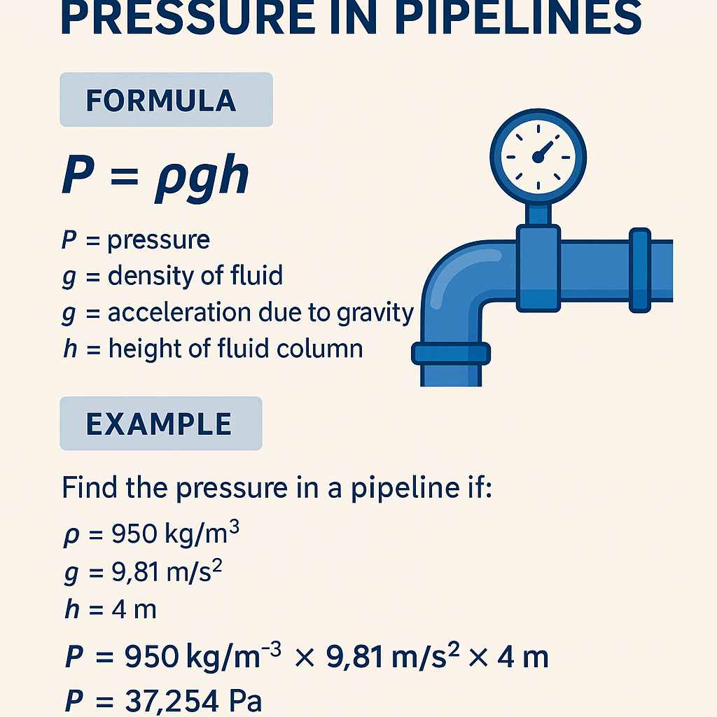
Hydrostatic pressure for a fluid column: P = ρ · g · h - P: pressure (Pa) - ρ: fluid density (kg/m³) - g: gravitational acceleration (9.80665 m/s²) - h: elevation difference (m) Typical values: - Water at 20 °C: ρ ≈ 998 kg/m³ - g = 9.80665 m/s² - Each 10 m head ≈ 98.07 kPa (0.9807 bar) Dynamic pressure: q = 0.5 · ρ · V² - q: dynamic pressure (Pa) - V: mean velocity (m/s) Frictional head loss (Darcy–Weisbach): h_f = f · (L/D) · (V² / (2 · g)) - h_f: head loss (m) - f: Darcy friction factor (dimensionless) - L: pipe length (m) - D: internal pipe diameter (m) Reynolds number (flow regime indicator): Re = (ρ · V · D) / μ - μ: dynamic viscosity (Pa · s) - Re < 2,300 usually laminar; Re > 4,000 turbulent.

Common fluid and pipe property tables

Friction factor estimation and Moody chart approximation

The Darcy friction factor f is a function of Re and relative roughness (ε/D). For turbulent flows, the Colebrook equation is implicit: 1 / √f = -2.0 log₁₀ ( (ε/(3.7 · D)) + (2.51 / (Re · √f)) ) Use explicit approximations for calculators: - Swamee–Jain: f = 0.25 / [log₁₀((ε/(3.7D)) + (5.74 / Re^0.9))]² Explain variables and typical ranges: - ε range: 10^-6 m (very smooth) to 10^-3 m (rough steel) - Re range: laminar (<2.3e3), transitional, turbulent (>4e3)

Design pressure calculation workflow

A robust pipeline pressure calculator should implement the following sequential checks and computations:

1. Define system boundaries: inlet pressure, outlet pressure, elevation profile, fluid properties.
2. Estimate mean velocity V = Q / A, where A = π · D² / 4.
3. Compute Re to select appropriate friction model.
4. Compute frictional losses (Darcy–Weisbach), and add losses for fittings using equivalent length or K-factors.
5. Account for static head changes due to elevation and pump/compressor boosts.
6. Apply safety factors and code-prescribed design margins per relevant standard (ASME, API, ISO).
7. Verify wall thickness and hoop stress using thin-wall or thick-wall cylinder formulas.

Hoop stress and minimum required wall thickness

For thin-walled cylinders (t < D/20), hoop stress: σ_h = (P · D) / (2 · t) Solve for t: t = (P · D) / (2 · σallow) - P: internal design pressure (Pa) - D: outside diameter (m) or use internal diameter depending on code - σallow: allowable stress (Pa), typically yield/ safety factor adjusted Typical allowable stresses: - Carbon steel allowable: σallow ≈ 0.6 · yield or per code (ASME B31.3 or B31.4 specify values)

Calculator affordability: essential features for practical implementers

An "affordable calculator" for pressure in pipelines must balance cost, accuracy, and usability. Essential features:

• Unit system flexibility (SI and imperial).
• Built-in property database (water, hydrocarbons, common chemicals) with temperature dependence.
• Friction models: laminar solution, Colebrook (iterative), Swamee–Jain (explicit), and empirical formulas for gases.
• Elevation/profile import (CSV/GPX) for head computation.
• Reports exportable to PDF/CSV with safety margin and code references.
• Audit trail and traceable inputs for regulatory compliance.

Regulatory and normative checks automated

Affordable calculators should embed normative checks to align with: - ASME B31.3 (Process Piping) and ASME B31.4 (Pipeline Transportation of Liquids) - API 5L (Line Pipe specifications) - ISO 3183 (Pipe for pipeline transportation systems) - AWWA standards for water distribution (C200, C900) - PHMSA/U.S. DOT guidance for gas/liquid transmission Include links for verification: - ASME: https://www.asme.org/ - API: https://www.api.org/ - ISO standards catalog: https://www.iso.org/ - U.S. PHMSA: https://www.phmsa.dot.gov/ - AWWA: https://www.awwa.org/

Formulas and variable tables with typical numerical values

Below are essential equations presented with variable explanations and typical values that affordable calculators must make accessible.

Real-world example 1: Water transmission main pressure and pump sizing

Problem statement: Design check for a 500 mm internal diameter ductile iron water transmission main transporting Q = 0.6 m³/s over L = 3,000 m. The inlet reservoir elevation is 30 m above sea level, outlet reservoir elevation is 15 m above sea level. Determine required pump head to overcome elevation and frictional losses. Use ρ = 998 kg/m³, viscosity μ = 1.002e-3 Pa·s, pipe roughness ε = 0.26 mm. Step 1 — compute cross-sectional area: A = π · D² / 4 = π · (0.5)² / 4 = 0.19635 m². Step 2 — mean velocity: V = Q / A = 0.6 / 0.19635 = 3.056 m/s. Step 3 — Reynolds number: Re = (ρ · V · D) / μ = (998 · 3.056 · 0.5) / 1.002e-3 ≈ 1.52e6 (turbulent). Step 4 — relative roughness: ε/D = 0.26e-3 / 0.5 = 5.2e-4. Step 5 — friction factor (Swamee–Jain explicit): f = 0.25 / [log₁₀((ε/(3.7·D)) + (5.74 / Re^0.9))]². Compute inside term: ε/(3.7D) = (0.26e-3) / (3.7·0.5) = 0.0001405. 5.74 / Re^0.9 ≈ 5.74 / (1.52e6)^0.9 ≈ 5.74 / (1.03e5) ≈ 5.57e-5. Sum ≈ 0.0001962. log₁₀(0.0001962) ≈ -3.707. f ≈ 0.25 / (-3.707)² ≈ 0.25 / 13.747 ≈ 0.01818. Step 6 — head loss (Darcy–Weisbach): h_f = f · (L/D) · (V² / (2 · g)) = 0.01818 · (3000 / 0.5) · (3.056² / (2 · 9.80665)) = 0.01818 · 6000 · (9.340 / 19.6133) = 0.01818 · 6000 · 0.4765 = 0.01818 · 2859 ≈ 52.03 m. Step 7 — total static head difference: Elevation difference = 30 - 15 = 15 m (pump must lift from lower to higher reservoir; assume pump at lower reservoir). Total required head = elevation lift + h_f + minor losses. Assume minor losses equivalent to 5% of h_f: K equiv. => add 2.6 m. Total head ≈ 15 + 52.03 + 2.6 = 69.63 m. Step 8 — required pump pressure (gauge): P = ρ · g · H = 998 · 9.80665 · 69.63 ≈ 680,300 Pa ≈ 0.6803 MPa (≈ 6.72 bar gauge). Design checks: - Check velocity recommended limits for water mains (often <3 m/s to limit erosion); here V = 3.056 m/s is slightly above typical; consider increase diameter or flow control. - Safety margin: select pump and pipe pressure class with >20% margin; round to 9 bar rated components. This full worked example illustrates how an affordable calculator automates each step and presents the final pump head and pressure in user-friendly units.

Real-world example 2: Crude oil pipeline internal pressure and wall thickness

Problem statement: Crude oil with density ρ = 860 kg/m³ flows through a buried steel pipeline with internal diameter D = 0.610 m at operating pressure P = 6 MPa. Determine minimum wall thickness t to keep hoop stress below allowable σallow = 150 MPa (per material and code margin). Step 1 — Use thin-wall hoop stress formula: σ_h = (P · D) / (2 · t) => t = (P · D) / (2 · σallow). Plug numbers: t = (6e6 Pa · 0.610 m) / (2 · 150e6 Pa) = (3.66e6) / (300e6) = 0.0122 m = 12.2 mm. Step 2 — Code allowances: - Corrosion allowance (CA): e.g., 1.5–3.0 mm depending on corrosion control. - Mill tolerance and fabrication: add +12.5% or as per standard. Applying CA = 2 mm: t = 12.2 + 2 = 14.2 mm. Applying fabrication tolerance of 12.5%: required t = 14.2 / (1 - 0.125) ≈ 16.23 mm. Round up to next standard plate thickness or pipe schedule: specify 18 mm nominal wall. Step 3 — Verify with Barlow's formula (alternative often used for pipes): P = (2 · σallow · t) / D -> rearranged same as hoop formula. Barlow often uses design factors; confirm with ASME/API factors. Step 4 — Additional checks: - Burst test and hydrostatic test pressure: apply test factor (e.g., 1.5 or 1.25 depending on code). - Longitudinal stress from axial loads, thermal expansion, and bending checks. This example shows how a pipeline pressure calculator must not only compute t from P, but also integrate corrosion allowance, fabrication tolerances, and code-prescribed test factors.

Compressible flow considerations and gas pipeline calculators

Gas pipelines require compressible flow models when pressure drops are significant relative to absolute pressure. Common engineering approaches:

• Use isothermal or adiabatic assumptions for line-sizing.
• Apply empirical formulas: Weymouth, Panhandle A/B, and AGA correlations for natural gas.
• For higher fidelity, solve one-dimensional compressible flow equations numerically (conservation of mass, momentum, and energy) with real gas properties from an equation of state.

An example of an approximate flow relation for steady, isothermal flow in a pipeline: dP/dx = - (ρ · f · V|V|) / (2 · D) But because ρ varies with P for gases, integrate along the line or use specialized calculators that implement the Weymouth or Panhandle formulae. References for gas pipeline calculations: - AGA (American Gas Association) reports - ISO 5167 for flow measurement - API and ASME pipeline specifications

Validation, uncertainty, and calibration for affordable calculators

An effective affordable pressure calculator must provide: - Uncertainty quantification for inputs (density, roughness, viscosity). - Sensitivity analysis to show how outcomes vary with input tolerances. - Calibration against field measurements (pressure transducers, flow meters). - Versioned documentation and normative references for auditability. Best practices:

1. Store default property values with references and date stamps.
2. Allow user-defined custom properties and save presets per project.
3. Include unit tests for core algorithms (Darcy–Weisbach, Swamee–Jain, Barlow).
4. Provide exportable calculation reports that list assumptions, coded margins, and normative citations.

Normative references and authoritative resources

Key normative sources and authoritative links that should be cited or embedded in a professional calculator:

• ASME B31.3 — Process Piping (https://www.asme.org/codes-standards)
• ASME B31.4 — Pipeline Transportation Systems for Liquids (https://www.asme.org/)
• API 5L — Specification for Line Pipe (https://www.api.org/)
• ISO 3183 — Petroleum and natural gas industries — Steel pipe for pipeline transportation systems (https://www.iso.org/)
• AWWA Standards (C200, C900) for water pipelines (https://www.awwa.org/)
• U.S. Pipeline and Hazardous Materials Safety Administration (PHMSA) guidance (https://www.phmsa.dot.gov/)
• NIST Chemistry WebBook for fluid properties (https://webbook.nist.gov/)

Implementation guidance for an affordable calculator

To make a practical, low-cost calculator suitable for international use, consider:

• Open-source core algorithms for friction and pressure checks to avoid licensing costs.
• Modular design: hydraulic engine, property database, code-check module, and report generator.
• Cloud-enabled for collaborative projects, with offline capability for field use.
• Localization of units and normative defaults per region (e.g., metric vs imperial, ASME vs EN annex choices).
• Security and audit logs for regulated industries.

UX considerations for engineers in the field

A useful affordable calculator must:

• Provide default templates for common scenarios (water main, crude pipeline, gas trunkline).
• Display intermediate results (Re, f, h_f) and enable step-by-step traceability.
• Offer graphical outputs: pressure profile vs. length, velocity profile, and margin-to-allowable stress.
• Allow import/export of elevation data and CAD coordinates for route-specific profiles.

Key mistakes to avoid and troubleshooting tips

Common pitfalls:

1. Mismatched units: SI vs imperial inconsistencies cause large errors.
2. Ignoring temperature dependence of viscosity and density, especially for oils and glycols.
3. Using inappropriate friction correlations for transitional flows.
4. Neglecting transient effects (water hammer) which may require surge analysis beyond steady-state calculators.

Troubleshooting approach:

• Verify inputs against literature values (NIST, manufacturer data).
• Perform order-of-magnitude sanity checks (e.g., head loss per km for water lines).
• Compare results with simplified formulas (hydrostatic checks) to find inconsistencies.

Final technical recommendations and adoption strategy

For organizations selecting or developing an affordable pipeline pressure calculator:

• Prioritize accuracy for the dominant physics (compressible vs incompressible, viscous dominated, etc.).
• Embed normative checks and provide links to the underlying clauses for design validation.
• Supply templates and training for engineers to guarantee consistent use across projects.
• Maintain a documented property database and algorithm validation against benchmark problems.

By combining validated hydraulic models (Darcy–Weisbach, Colebrook/Swamee–Jain), property libraries, and code-based safety margins, an affordable calculator becomes a practical engineering tool. It reduces design cycles, improves safety, and ensures compliance with international standards. References and further reading: - ASME codes and standards, ASME: https://www.asme.org/ - American Petroleum Institute standards, API: https://www.api.org/ - ISO standards catalogue, ISO: https://www.iso.org/ - U.S. PHMSA pipeline safety resources: https://www.phmsa.dot.gov/ - NIST Chemistry WebBook for precise fluid property data: https://webbook.nist.gov/ - AWWA standards and publications: https://www.awwa.org/ - "Fluid Mechanics" textbooks (e.g., White, Munson) for derivations and Moody chart background. Authoritative calculators and software examples (for benchmarking): - Open-source hydraulic libraries (search repositories for Darcy–Weisbach, Colebrook implementations). - Commercial pipeline simulation suites (use for validation; follow vendor documentation and licensing). Note: Use the formulas and worked examples above as templates when implementing or validating a pipeline pressure calculator. Ensure that final designs are reviewed by qualified engineers and cross-checked with the applicable codes listed in references.