This article quantifies instantaneous droop sharing for parallel synchronous and inverter-based generators under varying load.
Detailed calculator methodology, formulas, and worked examples determine each generator's share with precision during transients.
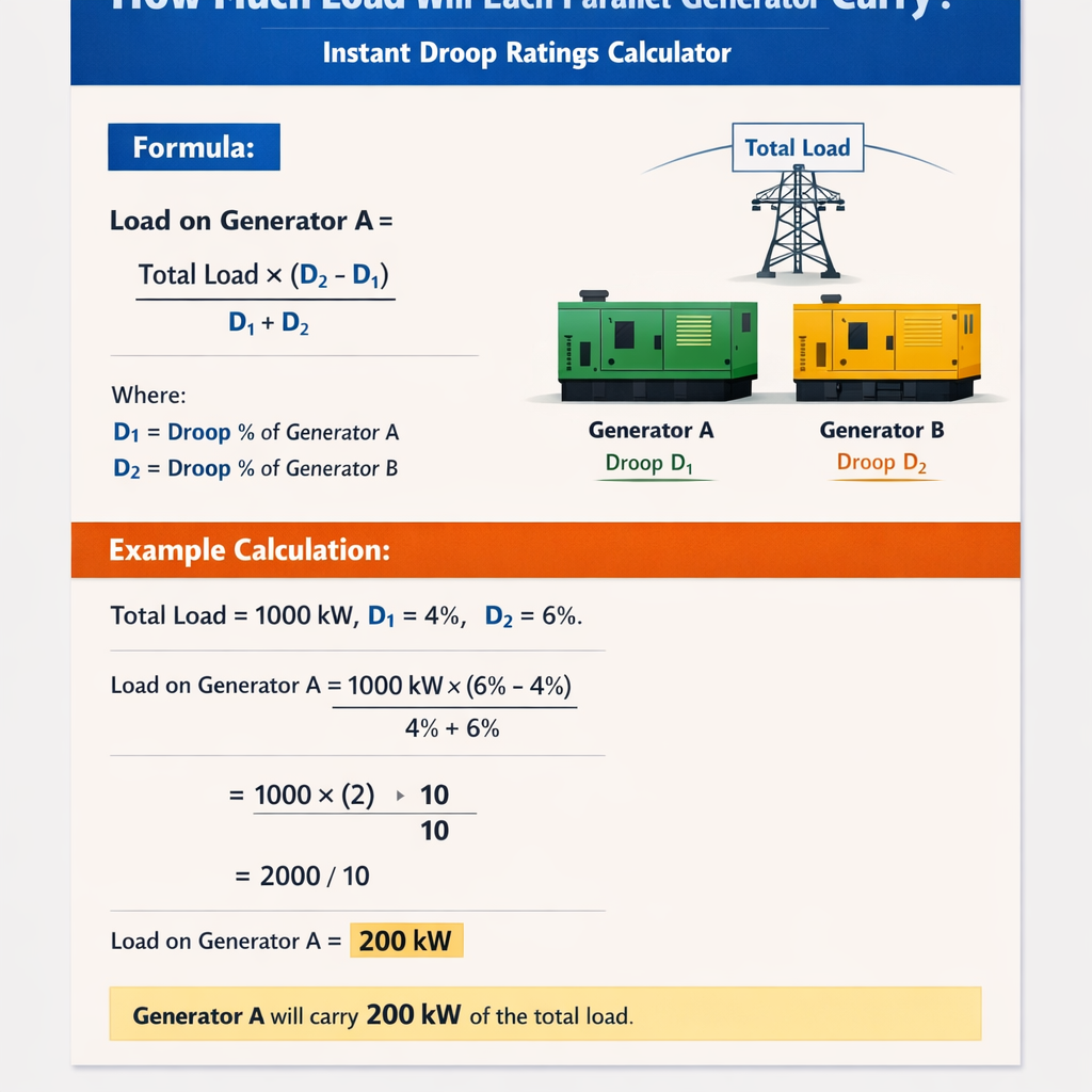
Instant Load Allocation among Parallel Generators using Droop Ratings (per-generator load share)
Fundamental principles of droop-based load sharing
Droop control is the predominant primary-frequency control strategy used to share sudden active-power changes among generators operating in parallel. The essential property is linear proportionality between frequency deviation and delivered power change: each unit changes its output in proportion to its droop constant. For a system-wide instantaneous load step, droop action produces a common frequency deviation Δf that sets the steady incremental power ΔP for each unit. Key assumptions for the following calculator approach:- All generators are connected to a common bus and measure the same system frequency.
- Each unit implements droop control that relates frequency deviation to change in active power (governor or inverter droop emulation).
- Reactive-power effects, voltage regulation, and time-delays are outside the steady instantaneous share calculation (they influence dynamics and stability but not the algebraic steady share).
Governing algebraic formulas and variable definitions
Use the droop relationships to derive each generator's share for a sudden total active-power change ΔP_total. Primary relations (expressed in plain HTML-friendly format):- ΔP_i: change in active power of generator i (MW or kW).
- ΔP_total: total change in system load (MW or kW). Positive for load increase; negative for load decrease.
- Δf: frequency deviation from nominal (Hz). Convention: Δf negative for load increase when using the sign convention above.
- R_i: droop constant of generator i expressed as power change per Hz (MW/Hz or kW/Hz). R_i can be computed from %droop using rated power and system nominal frequency.
- %droop_i: manufacturer or setting percentage, e.g., 4% means full-load causes Δf = 0.04 * f_nom.
- f_nom: nominal system frequency (50 Hz or 60 Hz).
- Small diesel gen-set: droop 4%–6%, rated power 50 kW–2 MW.
- Large steam turbine: droop 3%–5%, rated power 10 MW–1500 MW.
- Inverter-based DG emulation: configurable droop, typically 3%–5% for active-power sharing.
Practical calculator algorithm (step-by-step)
Follow these steps to calculate instantaneous load share using droop parameters:- Collect generator data: RatedPower_i, %droop_i, nominal frequency f_nom, and current operating points (pre-step outputs P_i0 and headroom limits).
- Convert %droop_i to R_i (power/Hz) using R_i = RatedPower_i / (f_nom * (%droop_i/100)).
- Sum the stiffness terms: S = Σ_i (1 / R_i).
- Compute Δf = -ΔP_total / S (units: Hz).
- Compute ΔP_i = (1 / R_i) * (-Δf) = (1 / R_i) / S * ΔP_total for each i.
- Check generator limits: if |P_i0 + ΔP_i| > RatedPower_i or below minimum, clamp that generator to its limit and remove it from the free-share set; recalculate S and distribute the remainder iteratively among remaining generators.
- Report final P_i = P_i0 + ΔP_i for each generator and the common Δf.
Limit handling and iterative reallocation procedure
When a generator reaches its maximum or minimum capability during the computed share, the assumptions for linear distribution no longer hold. Implement this iterative algorithm:- Compute initial shares for all units.
- Find any unit where P_i0 + ΔP_i exceeds rating bounds.
- Fix those units at their bound (saturated). Remove them from the share pool and reduce ΔP_total by the amount allocated to the saturated units.
- Recompute S = Σ over remaining units (1 / R_i), recompute Δf and ΔP_i for remaining units.
- Repeat until no further saturation occurs or all units are saturated.
Tables: common generator ratings, droop settings and derived R constants
| Rated Power | % Droop | Nominal f (Hz) | Δf_fullscale (Hz) | R (power/Hz) | R (kW/Hz) |
|---|---|---|---|---|---|
| 50 kW | 4% | 50 | 2.00 | 25 kW/Hz | 25 |
| 100 kW | 5% | 50 | 2.50 | 40 kW/Hz | 40 |
| 500 kW | 4% | 50 | 2.00 | 250 kW/Hz | 250 |
| 1 MW | 5% | 50 | 2.50 | 400 kW/Hz | 400 |
| 2 MW | 4% | 50 | 2.00 | 1000 kW/Hz | 1000 |
| 10 MW | 5% | 50 | 2.50 | 4000 kW/Hz | 4000 |
| 100 MW | 4% | 50 | 2.00 | 50 000 kW/Hz | 50 000 |
| 100 MW | 5% | 60 | 3.00 | 33 333 kW/Hz | 33 333 |
| 500 MW | 3% | 60 | 1.80 | 277 778 kW/Hz | 277 778 |
| Generator Type | Typical % Droop | Application | Notes |
|---|---|---|---|
| Diesel genset | 4%–6% | Islanded microgrids, standby | Good primary frequency response, robust |
| Steam turbine | 3%–5% | Large thermal plant, grid support | Lower droop for stiffer participation |
| Gas turbine | 3%–5% | Peaking/combined cycle | Fast response if turbine speed control tuned |
| Inverter (droop emulation) | 0%–6% | DER, PV+storage, microgrids | Configurable; can implement virtual inertia |
Worked example 1: Two synchronous generators with identical droop
System description:- Generator A: RatedPower_A = 2.0 MW, %droop_A = 4.0%, f_nom = 50 Hz, initial P_A0 = 1.0 MW.
- Generator B: RatedPower_B = 1.0 MW, %droop_B = 4.0%, initial P_B0 = 0.5 MW.
- Sudden load increase: ΔP_total = +1.5 MW.
For both generators: Δf_fullscale = f_nom * (%droop / 100) = 50 * 0.04 = 2.00 Hz.
R_A = RatedPower_A / Δf_fullscale = 2.0 MW / 2.0 Hz = 1.0 MW/Hz.
R_B = 1.0 MW / 2.0 Hz = 0.5 MW/Hz.
Step 2 — compute stiffness S = Σ(1 / R_i):P_B = 0.5 + 1.0 = 1.5 MW, but this exceeds Generator B rated power of 1.0 MW so B saturates.
Step 6 — handle saturation iteratively:- Generator B is limited to 1.0 MW. It can only increase by 0.5 MW from 0.5 MW to 1.0 MW.
- Remaining required increase after B saturates: ΔP_remaining = 1.5 MW - 0.5 MW (provided by B) = 1.0 MW.
- Only Generator A remains free to provide the remaining 1.0 MW increase. Check its available headroom: RatedPower_A - P_A0 = 2.0 - 1.0 = 1.0 MW available, so A can supply the remainder.
Δf = -ΔP_total / Σ_active(1 / R_active) where the active set before final saturation is A only for the last increment. Numerically the realized Δf in the final saturated solution is determined by the portions of output reachable given limits and governor droops; the simplest reporting is final P_i values and that governors are saturated.
Key learning: identical droop percentages do not guarantee proportional power by rating; the ratio is determined by R_i which depends both on %droop and rated power.Worked example 2: Heterogeneous park with iterative redistribution
System description:- Generator 1 (G1): Rated 5.0 MW, %droop 5.0%, P1_0 = 2.0 MW.
- Generator 2 (G2): Rated 2.0 MW, %droop 3.0%, P2_0 = 0.5 MW.
- Generator 3 (G3, inverter): Rated 1.0 MW, %droop 4.0%, P3_0 = 0.0 MW (on standby).
- Nominal f = 50 Hz. Load step ΔP_total = +4.0 MW.
- G1 final P1 = 2.0 + 0.615 = 2.615 MW (within 5.0 MW).
- G2 final P2 = 0.5 + 0.923 = 1.423 MW (within 2.0 MW).
- G3 final P3 = 0.0 + 2.462 = 2.462 MW which exceeds G3 rating 1.0 MW → saturates.
- G3 can only provide 1.0 MW of the requested 2.462 MW, contributing ΔP3_actual = 1.0 MW.
- Already supplied by G3: 1.0 MW. Remaining load to allocate: ΔP_remaining = 4.0 - 1.0 = 3.0 MW.
- Remove G3 from pool. Recompute S for active units G1 and G2: S_new = (1 / R1) + (1 / R2) = 0.5 + 0.75 = 1.25 Hz/MW.
- Δf_new = -ΔP_remaining / S_new = -3.0 / 1.25 = -2.4 Hz.
- ΔP1_new = (1 / R1) / S_new * ΔP_remaining = 0.5 / 1.25 * 3.0 = 1.2 MW.
- ΔP2_new = 0.75 / 1.25 * 3.0 = 1.8 MW.
P2_final = 0.5 + 1.8 = 2.3 MW → exceeds G2 rating 2.0 MW so G2 saturates at 2.0 MW
Step 8 — second iteration after G2 saturation:- G2 can supply only ΔP2_actual = 2.0 - 0.5 = 1.5 MW. Total supplied so far: G3 1.0 + G2 1.5 = 2.5 MW. Remaining required: ΔP_remaining2 = 4.0 - 2.5 = 1.5 MW.
- Only G1 remains free. G1 available headroom: 5.0 - 2.0 = 3.0 MW, so it can supply the remaining 1.5 MW.
- P1_final = 2.0 + 1.5 = 3.5 MW.
- G1 final = 3.5 MW (within rating)
- G2 final = 2.0 MW (saturated)
- G3 final = 1.0 MW (saturated)
- System frequency deviation in the final saturated steady state will be consistent with G1 providing leftover increment and the saturated units at their limits; the effective Δf is the final governor deviation required for G1 to produce 1.5 MW: Δf_final = -ΔP1_actual / (1 / (1/R1)?), but practically frequency is determined by the mismatched droop behaviour and saturations. Reporting final P_i and saturated flags is the required result for operational planning.
Effects of differing nominal frequency and percent droop definitions
Remember that %droop definitions are relative to nominal frequency. For example:- At 50 Hz, 5% droop corresponds to Δf_fullscale = 2.5 Hz.
- At 60 Hz, 5% droop corresponds to Δf_fullscale = 3.0 Hz.
R = RatedPower / (f_nom * (%droop / 100)).
A generator set described with %droop but without explicit nominal frequency requires a consistent f_nom to compute R.Frequency response characteristics, dynamics and limitations
While the algebra above determines instantaneous proportional sharing for primary droop, several dynamic and practical factors affect the real-world response:- Governor time constants and actuator delays produce a temporal evolution toward the algebraic steady share; the initial instant may be dominated by governor deadband or inverter control loop dynamics.
- Inverter-based resources can emulate droop with configurable virtual inertia; their effective R_i may change as control tuning changes.
- Speed governors and power control loops may include deadband and rate-limiting; deadband causes no change in output for small Δf, complicating sharing for small disturbances.
- System inertia does not change steady-state algebraic distribution but affects how fast the system moves to that steady state, and how much the nadir frequency deviates during transients.
- Protection and anti-islanding settings on DERs may trip units under large Δf; the calculator must be used together with protection coordination studies.
Implementation considerations for a calculator tool
Key software features to include for a robust droop-sharing calculator:- Input validation: unit ratings, current outputs, droop percent, nominal frequency, and per-unit or MW units consistency checks.
- Unit conversion utilities: convert %droop to R (MW/Hz), support kW and MW inputs transparently.
- Iterative saturation solver to handle generator limits and priority dispatch rules.
- Transient approximation: optional governor time-constant based estimate for frequency nadir and time to reach steady share (simple first-order models).
- Reporting: final P_i, Δf, saturation flags, and recommended actions if limits violated.
Example calculation flow (pseudo-procedure)
- Step 0: Read generator array G[i] with fields: RatedPower, P0, %droop, minP, maxP.
- Step 1: For each i compute R_i and stiffness k_i = 1 / R_i.
- Step 2: ActiveSet = all units not at limits.
- Step 3: While ΔP_remaining != 0 and ActiveSet not empty: compute S = Σ k_i for ActiveSet, Δf = -ΔP_remaining / S, ΔP_i = k_i / S * ΔP_remaining for i in ActiveSet. If any ΔP_i would push P_i out of [minP,maxP], clamp, update ΔP_remaining and ActiveSet.
- Step 4: Output final P_i and Δf (the final Δf can be reported computed from the active set at the last iteration).
Standards, normative guidance and authoritative references
For design and interconnection, consult the following standards and technical references:- IEEE Std 1547 series — Interconnection and interoperability of distributed resources with power systems: https://standards.ieee.org/standard/1547-2018.html
- EN 50549 — Requirements for connection of generation to distribution networks (European DER connection rules): https://standards.cencenelec.eu/
- IEC 60034 — Rotating electrical machines (general performance and testing guidance): https://www.iec.ch/
- NERC Reliability Standards — for balancing and frequency control practices: https://www.nerc.com/
- Kundur, P., Power System Stability and Control — classical textbook covering governor-droop and stability topics.
- NREL and technical papers on droop control and inverter-based resources: https://www.nrel.gov/
Practical recommendations and best practices for engineers
- Use droop sharing calculators during commissioning to verify expected participation factors and headroom requirements under plausible contingencies.
- Set droop percentages intentionally to reflect capacity and desired participation; do not assume uniform %droop across disparate machine ratings will yield proportional power by rating.
- Account for dynamic responses: combine droop-sharing algebra with time-constant models to estimate frequency nadirs and peak power during the transient.
- Implement limit-checking and anti-windup mechanisms in governors and inverter controllers to prevent integrator saturation and unacceptable frequency excursions.
- Document and log actual responses during initial load steps so that model parameters (effective R_i and time constants) can be validated and tuned.
SEO-oriented summary of key formulas and keywords for quick reference
For rapid calculation:Final technical notes and limitations
The algebraic droop-sharing approach calculates steady-state distribution that primary frequency control tends to settle on after a disturbance, but:- Transient inertial response and governor dynamics determine the frequency nadir and time to steady-state; include inertia modeling for full transient studies.
- Reactive-power sharing, voltage regulation, and AGC/secondary control layers interact with primary droop and must be coordinated.
- In microgrids switching between grid-connected and islanded modes may require changing droop configurations (e.g., enabling inverter droop only when islanded).
- Protection settings and low/high frequency trip settings must be checked to prevent inadvertent disconnection during droop events.