The design and verification of electrical cables demand rigorous understanding of thermal dissipation mechanisms and losses. Every conductor produces electrical resistance, dielectric, and proximity losses, manifesting as heat; proper calculation ensures safety.
Thermal Dissipation Calculator — Electrical Cables (I²R & temp rise)
What inputs give most accurate results?
What is thermal resistance (R_th) and how to choose it?
Why does resistance increase with temperature?
Extended Reference Table — Common Thermal Dissipation Values
The following table compiles typical values used in thermal dissipation analysis for electrical cables. These values are drawn from IEC standards, NEC guidelines, and engineering handbooks. They serve as reference starting points; real projects require site-specific adjustments.
| Parameter | Symbol | Typical Range / Value | Units | Notes |
|---|---|---|---|---|
| Electrical resistivity of copper (20°C) | ρ_Cu | 1.72 × 10⁻⁸ | Ω·m | Increases ~0.39%/°C |
| Electrical resistivity of aluminum (20°C) | ρ_Al | 2.82 × 10⁻⁸ | Ω·m | Lighter but higher resistance |
| Temperature coefficient of copper | α_Cu | 0.00393 | 1/°C | Linear approx. up to 150°C |
| Conductor resistance per km (Cu, 25 mm², 20°C) | R20 | 0.727 | Ω/km | Source: IEC 60228 |
| Conductor resistance per km (Al, 25 mm², 20°C) | R20 | 1.20 | Ω/km | Higher losses |
| Permissible continuous conductor temperature (PVC) | θ_max | 70 | °C | Per IEC 60287 |
| Permissible continuous conductor temperature (XLPE) | θ_max | 90 | °C | Common in power cables |
| Permissible emergency temperature (XLPE) | θ_em | 130 | °C | Short-term overload |
| Permissible short-circuit temperature (XLPE, 1s) | θ_sc | 250 | °C | Withstand thermal stress |
| Soil thermal resistivity (average) | ρ_th | 1.0–1.5 | K·m/W | Strongly site dependent |
| Air thermal resistivity (natural convection) | ρ_th,air | 0.3–0.4 | K·m/W | Approximation |
| Heat transfer coefficient — air (natural convection) | h | 5–25 | W/m²·K | Depends on installation |
| Heat transfer coefficient — forced air | h | 25–250 | W/m²·K | With ventilation |
| Heat transfer coefficient — buried cables (soil) | h_soil | 0.5–1.5 | W/m²·K | Influenced by moisture |
| Stefan–Boltzmann constant | σ | 5.67 × 10⁻⁸ | W/m²·K⁴ | For radiation calc. |
| Surface emissivity (PVC sheath) | ε | 0.92 | – | Dark surfaces, high emissivity |
| Surface emissivity (PE sheath) | ε | 0.85 | – | Slightly lower |
| Specific heat of copper | c_Cu | 385 | J/kg·K | Used in transient heating |
| Density of copper | ρ_m,Cu | 8960 | kg/m³ | Required for short-circuit thermal limit |
This table provides baseline data used in steady-state and transient thermal dissipation calculations.
Core Formulas for Thermal Dissipation in Electrical Cables
1. Joule Heating (I²R Losses)
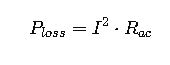
- P_loss = Heat generated per unit length [W/m]
- I = Current through conductor [A]
- R_ac = AC resistance per unit length at operating temperature [Ω/m]
Note: Rac accounts for skin effect and proximity effect in AC conditions.
Common values:
- For small conductors (<10 mm², <60 Hz), AC resistance ≈ DC resistance.
- For large conductors (>300 mm²), correction factors can increase resistance by 10–20%.
2. Resistance at Operating Temperature
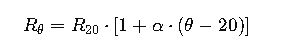
- R_θ = Resistance at temperature θ [Ω/m]
- R_20 = Resistance at 20°C [Ω/m]
- α = Temperature coefficient [1/°C]
- θ = Operating temperature [°C]
3. Heat Balance Equation (Steady State)
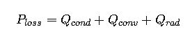
Where:
- Q_cond = Heat conducted through soil, duct, or insulation [W/m]
- Q_conv = Heat dissipated by convection to air/fluids [W/m]
- Q_rad = Radiated heat from cable surface [W/m]
4. Convection Heat Transfer
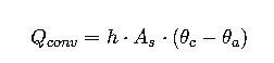
- h = Heat transfer coefficient [W/m²·K]
- A_s = Cable surface area per unit length [m²/m] = π·D
- θ_c = Cable surface temperature [°C]
- θ_a = Ambient temperature [°C]
5. Radiation Heat Transfer

- ε = Emissivity (dimensionless, 0–1)
- σ = Stefan–Boltzmann constant (5.67 × 10⁻⁸ W/m²·K⁴)
- A_s = Cable surface area per unit length [m²/m]
- T_c = Cable surface absolute temperature [K]
- T_a = Ambient absolute temperature [K]
6. Conduction Through Surroundings (Buried Cables)
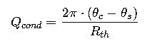
Where:
- θ_c = Cable surface temperature [°C]
- θ_s = Soil temperature [°C]
- R_th = Thermal resistance per unit length [K·m/W]
Approximate soil thermal resistance:
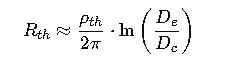
- ρ_th = Soil thermal resistivity [K·m/W]
- D_e = Equivalent thermal diameter of burial environment [m]
- D_c = Cable diameter [m]
7. Current Rating (Ampacity) Based on Thermal Balance
From IEC 60287, the permissible current is:
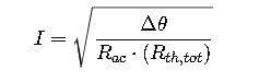
- I = Maximum continuous current [A]
- Δθ = Temperature rise allowed (θ_max − θ_amb) [K]
- R_ac = Conductor AC resistance at θ_max [Ω/m]
- R_th,tot = Total thermal resistance (conduction + convection + radiation) [K·m/W]
Key Variables Influencing Thermal Dissipation in Electrical Cables
While mathematical models are essential, understanding the physical meaning and practical range of each variable allows engineers to apply calculations effectively. Below are the most relevant parameters, explained in detail.
1. Conductor Material
- Copper (Cu):
- Lower resistivity, hence lower I²R losses.
- Higher density and cost.
- Preferred in critical installations requiring compact design.
- Aluminum (Al):
- Higher resistivity (≈65% more than copper).
- Lighter weight, lower cost.
- Widely used in transmission and distribution.
Impact on thermal dissipation: Aluminum cables generate more heat per ampere but may dissipate faster due to larger diameters.
2. Insulation Type
The insulation material limits the maximum operating temperature.
| Insulation Material | Typical Max Continuous Temperature | Emergency Overload Temperature | Short-Circuit Limit |
|---|---|---|---|
| PVC | 70 °C | 100 °C | 160 °C |
| XLPE | 90 °C | 130 °C | 250 °C |
| EPR | 90–105 °C | 140 °C | 250 °C |
| Paper-Insulated (PILC) | 80 °C | 105 °C | 160–200 °C |
Impact: XLPE insulation dominates modern power cables due to higher permissible temperatures and better thermal stability.
3. Installation Method
Heat dissipation strongly depends on where the cable is installed:
- Buried in soil: Limited convection, conduction dominates. Soil thermal resistivity is critical.
- In conduit: Conduction through the conduit plus possible convection if ventilated.
- Free air (open trays, ladders): Convection and radiation dominate, often allowing higher ampacities.
- Grouped cables: Mutual heating reduces dissipation efficiency. De-rating factors apply.
4. Ambient and Surrounding Conditions
- Soil thermal resistivity: Dry sandy soil may reach 2.5 K·m/W, while moist clay can be as low as 0.8 K·m/W.
- Ambient air temperature: Often 30–40 °C in design standards, but tropical sites may exceed 45 °C.
- Airflow conditions: Forced ventilation drastically improves dissipation.
5. Cable Surface and Emissivity
- Dark PVC or PE sheaths: High emissivity (~0.9), enhancing radiation cooling.
- Metallic or light-colored surfaces: Lower emissivity, more reliance on convection.
Reference Tables for Practical Engineering
Typical Current Density Guidelines (Safe Operating Ranges)
| Conductor Material | Typical Current Density in Air (A/mm²) | In Buried Conditions (A/mm²) |
|---|---|---|
| Copper | 2.5–4.0 | 1.5–2.5 |
| Aluminum | 1.5–2.5 | 1.0–1.8 |
Values are general rules of thumb; standards (IEC 60287, NEC) provide exact ratings.
Soil Thermal Resistivity Influence on Ampacity
| Soil Thermal Resistivity (K·m/W) | Relative Ampacity (%) |
|---|---|
| 0.8 (moist clay) | 120% |
| 1.0 (average soil) | 100% |
| 1.5 (dry sand) | 75% |
| 2.5 (very dry soil) | 50% |
Engineering note: Seasonal variation in soil moisture can drastically change cable performance. Utilities often assume conservative values (1.5 K·m/W) to ensure safety.
Real-World Application Cases
Case Study 1 — Industrial Plant Cable in Free Air
Scenario:
An industrial facility installs 240 mm² copper XLPE cables on ladder trays. Ambient air temperature is 35 °C, and cables are installed with spacing to allow air circulation.
Steps Taken by Engineers:
- Conductor material: Copper, ensuring low resistance.
- Insulation limit: XLPE allows 90 °C continuous operation.
- Heat dissipation mode: Mainly natural convection and radiation.
- Design adjustment: Spacing between cables increased to prevent mutual heating.
Result:
- Calculated ampacity ≈ 500–520 A per cable.
- Verified against IEC 60287 tables and manufacturer datasheets.
- Operating current set at 470 A (≈90% capacity) for long-term reliability.
Lesson Learned:
Free-air installations allow higher currents due to efficient convection and radiation, but ambient conditions and spacing remain decisive.
Case Study 2 — High-Voltage Feeder Buried in Soil
Scenario:
A utility company installs 1000 mm² aluminum XLPE single-core cables in a trench, at 1 m burial depth. Soil thermal resistivity is 1.5 K·m/W, and ambient soil temperature is 25 °C.
Steps Taken by Engineers:
- Conductor material: Aluminum selected for cost and weight savings.
- Insulation type: XLPE allows 90 °C operation.
- Soil properties: High thermal resistivity reduces dissipation capacity.
- Thermal analysis: Using IEC 60287, ampacity reduced due to soil conditions.
- Mitigation measure: Engineers added a sand backfill with ρ_th = 1.0 K·m/W to improve dissipation.
Result:
- Initial ampacity (dry soil, 1.5 K·m/W) ≈ 850 A.
- After backfilling with better soil (1.0 K·m/W), ampacity improved to ≈ 1000 A.
Lesson Learned:
Environmental conditions dominate buried cable performance. Proper soil treatment is often more cost-effective than oversizing conductors.