This article presents a rapid transformer temperature rise screening calculator and risk estimation methodology overview.
Engineers will learn inputs, formulas, example calculations, and risk thresholds for operational load profiles assessment.
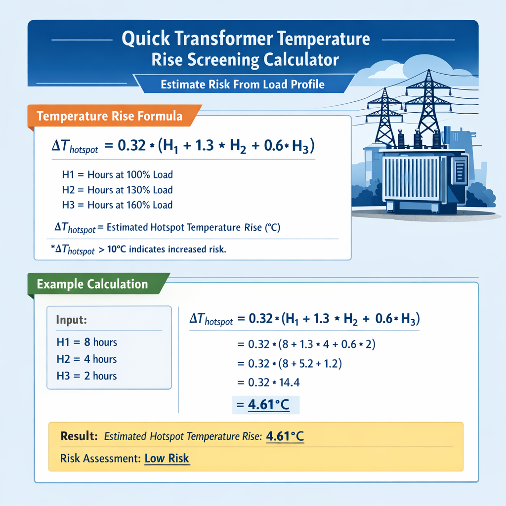
Quick Transformer Temperature Rise Screening — Estimate Hotspot Temperature and Risk from Load Profile
Purpose and scope of the quick screening calculator
This technical guide defines a rapid, deterministic screening method to estimate transformer temperature rise and export a simple risk indicator from a given load profile. It targets engineers who need fast, conservative evaluations to prioritize field thermal studies and identify likely overload or accelerated-aging scenarios.
Thermal model fundamentals and assumptions
Basic electrical and thermal relationships
Key scalar definitions and the fundamental steady-state relationships used in screening:
- Load factor K = I / I_rated (per unit current or per unit load).
- Load losses scale with current squared: P_load(K) = P_load,rated × K^2.
- Top-oil temperature rise steady-state scales roughly with combined load and loss distribution using empirical exponents.
Core screening formulas (HTML notation)
1) Load factor:
2) Steady-state top-oil temperature-rise (empirical):
3) Steady-state winding hottest-spot temperature-rise above top-oil:
4) Transient response (first-order approximation) for top-oil:
5) Transient response for hottest-spot (winding) relative to its steady-state value:
6) Absolute temperatures (ambient based):
Variable definitions and typical engineering values
- Δθ_TO,R — rated top-oil rise above ambient at rated load. Typical: 45°C to 65°C (commonly 55°C for many distribution units).
- Δθ_H,R — rated hottest-spot (winding) rise above top-oil at rated load. Typical: 20°C to 40°C (commonly 30°C).
- R — ratio of rated load losses to no-load losses: R = P_load,rated / P_no-load. Typical: 2 to 12 depending on size and design (smaller distribution units ~3–6; large power transformers ~8–15).
- n — oil heating exponent for top-oil steady-state: typical values 0.8 to 1.0 (0.8 commonly used for ONAN natural convection).
- m — winding exponent for hottest-spot: typical 0.8 to 1.0 (0.8 commonly used).
- τ_TO — top-oil thermal time constant. Typical range: 1.5 h (small units) to 6 h (large power transformers). Common conservative value: 3–4 h.
- τ_H — winding (hotspot) time constant. Typical 0.3 h to 1.5 h (often 0.5–1.0 h).
- θ_A — ambient temperature (°C) during evaluation. Use measured or design ambient (e.g., 20°C, 30°C, 40°C for hot climates).
- θ_HS — hottest-spot absolute temperature (°C), used for insulation aging assessment.
Tables of typical transformer parameters and thresholds
| Rating (approx) | Cooling type | Δθ_TO,R (°C) | Δθ_H,R (°C) | R (Pload/ Pno-load) | τ_TO (h) | τ_H (h) |
|---|---|---|---|---|---|---|
| 50 kVA (pole-mounted) | ONAN | 55 | 30 | 3 | 1.5 | 0.5 |
| 250 kVA (pad-mounted) | ONAN | 55 | 30 | 4 | 2.0 | 0.6 |
| 500 kVA (industrial) | ONAN | 55 | 30 | 5 | 3.0 | 0.8 |
| 2 MVA (substation) | ONAN/ONAF | 45 | 28 | 6 | 4.0 | 1.0 |
| 20 MVA (power) | ONAF/ONAN | 40 | 25 | 8 | 5.0 | 1.2 |
| Insulation class | Maximum winding temperature (°C) | Notes |
|---|---|---|
| A | 105 | Historic cellulose rating; limited modern use |
| E/F | 130–155 | Common modern thermal classes (F = 155°C) |
| H | 180 | High-temperature insulation, used for some classes |
| Oil thermal limit | ~105–120 | Oil flash/oxidation concerns; keep below recommended values |
Screening algorithm: from load profile to risk bands
High-level screening steps
- Collect inputs: transformer rated parameters (Δθ_TO,R, Δθ_H,R, R, τ_TO, τ_H, rated current), ambient temperature time series, and the measured or estimated load profile (hourly or finer resolution).
- Convert load profile to per-unit load K(t) = load(t) / rated_load.
- At each time step compute steady-state Δθ_TO,ss(t) and Δθ_H,ss(t) from K(t) using the empirical formulas.
- Simulate transient temperature using first-order time constants and the prior step value (discrete-time exponential update), producing Δθ_TO(t) and Δθ_H(t).
- Compute absolute temperatures θ_HS(t) = θ_A(t) + Δθ_TO(t) + Δθ_H(t).
- Compare θ_HS against insulation thresholds and derive a risk indicator (low/medium/high). Also determine if predicted steady-state or transient exceedance of specified limits is possible.
- Flag periods where hottest-spot temperature is close to or exceeds limit, and prioritize for detailed dynamic thermal FEM or monitored testing.
Discrete-time update equations for a time-step Δt
Given Δt (hours), previous top-oil rise Δθ_TO(prev) and target Δθ_TO,ss:
Use Δt equal to the sampling interval of the load profile (e.g., 1 hour, 15 minutes). Initialize Δθ_TO(0) and Δθ_H(0) to ambient steady-state at the initial K.
Risk indicators, aging rate estimation and screening thresholds
Common engineering screening bands (conservative):
- Low risk: θ_HS,max ≤ 95% of insulation class limit.
- Moderate risk: 95% < θ_HS,max ≤ 100% of limit — requires monitoring or seasonal derating.
- High risk: θ_HS,max > 100% — immediate investigation, potential load reduction, or cooling upgrade.
Approximate aging acceleration factor follows Arrhenius-like relation for insulation: a rule-of-thumb doubles aging per 6–7°C rise at hot-spot above a reference (commonly 98°C reference for IEEE/IEC aging factors). For screening use conservative multiplier table:
| θ_HS (°C) | Relative aging rate (approx) | Screening implication |
|---|---|---|
| < 90 | ≤ 0.5× | Minimal accelerated aging |
| 90–110 | 0.5–2× | Manageable; monitor |
| 110–130 | 2–10× | Moderate to high aging; derate recommended |
| >130 | >10× | Severe accelerated aging; urgent action |
Example calculations — practical cases
Below are two fully developed examples illustrating the full workflow, assumptions, and numeric outputs.
Example 1 — 500 kVA pad-mounted distribution transformer, step-load event
Given data and assumptions:
- Transformer rating: 500 kVA, 11 kV/400 V, ONAN.
- Δθ_TO,R = 55°C, Δθ_H,R = 30°C.
- R = 5 (P_load,rated / P_no-load).
- n = 0.8, m = 0.8.
- τ_TO = 3.0 h, τ_H = 0.8 h.
- Ambient θ_A = 30°C (constant).
- Load profile: steady at 0.6 p.u. for long time, then step to 1.2 p.u. at t = 0 and holds.
- Initial steady-state prior to step: K_initial = 0.6.
Step 1 — compute steady-state rises before step (initial steady-state):
Initial hottest-spot absolute temperature θ_HS0 = θ_A + Δθ_TO,ss0 + Δθ_H,ss0 = 30 + 29.5 + 13.2 = 72.7 °C
Raise to 0.8: 1.366667^0.8 ≈ 1.292
This steady-state exceeds common insulation limits (e.g., 155°C H-limit maybe still above but for class F 155°C; for class A/E this is far above). It predicts severe accelerated aging if maintained.
Step 3 — transient response after t hours using first-order model. Calculate after 2 hours and 6 hours as sample:
Initiate Δθ_TO(0) = Δθ_TO,ss0 = 29.5 °C; Δθ_H(0) = 13.2 °C.
e^(−2/3) ≈ e^(−0.6667) ≈ 0.5134
e^(−7.5) ≈ 0.000553 → Δθ_H(6h) ≈ 40.14 − 0.0149 ≈ 40.12 °C
Screening result summary (Example 1):
- Initial θ_HS = 72.7°C (safe).
- After 2 hours at 1.2 p.u., θ_HS ≈ 118°C (moderate to high aging).
- After 6 hours, θ_HS ≈ 136°C (severe accelerated aging; approach insulation class F limit ≈155°C).
- Steady-state at 1.2 p.u. would be 141°C (high risk; immediate mitigation recommended if sustained loads reach 1.2 p.u.).
Actions: apply load shedding, investigate forced cooling (ONAF), or reduce loading duration to limit cumulative thermal aging.
Example 2 — 20 MVA substation transformer with cyclic daily profile (24-hour simulation)
Given data and assumptions:
- Rating: 20 MVA, load losses high (R = 8), Δθ_TO,R = 40°C, Δθ_H,R = 25°C.
- n = 0.9, m = 0.8, τ_TO = 5.0 h, τ_H = 1.2 h.
- Ambient temperature daily profile (°C): 18 at 03:00, ramp to 30 at 15:00, back to 18 at 23:00 (hourly values provided).
- Load profile hourly K(t): 0.5 (night 00–06), ramp to 1.0 (08–18 peak), dip to 0.8 evening (18–22), then 0.6 overnight.
- Time-step Δt = 1 hour. Initialize at steady-state for 0.5 p.u. at t = 0.
θ_HS0 initial at ambient 18°C: θ_HS0 = 18 + 14.56 + 8.25 = 40.81 °C (very safe).
Step 2 — run hourly discrete simulation for 24 hours. We show selected hours and compute method. For brevity show steps: hours 0→1→... and results at key times (08:00, 15:00 peak, 22:00).
Δθ_TO,ss(1.0) = 40 × ((1^2 × 8 + 1) / 9)^0.9 = 40 × (9/9)^0.9 = 40 × 1 = 40 °C
e^(−1/5) ≈ 0.8187
Continue simulation to 15:00 peak (several hours at K=1.0 and ambient 30°C). After many hours Δθ_TO and Δθ_H will approach the steady-state 40 and 25 respectively; time constants indicate Δθ_TO will reach ~95% in ~3×τ_TO = 15 h, but with several hours at full load significant rise occurs. Example at 15:00 (7 hours after 08:00): cumulative update using exponential closed-form from initial Δθ_TO at 08:00:
Δθ_H(15:00) = 25 + (17.66 − 25) × e^(−7/1.2) ; e^(−5.833) ≈ 0.00292 → Δθ_H(15) ≈ 25 − 0.023 ≈ 24.98 °C
Even at 15:00 peak the hottest-spot is below aggressive aging thresholds (approx 90°C). At 18:00 K drops to 0.8 and ambient begins to fall; cooling will begin and temperatures will decline over time. Maximum θ_HS in the day in this scenario ~90°C.
Screening result summary (Example 2):
- Transient and steady-state peak hottest-spot ≈ 90°C (low to moderate aging; acceptable for many installations).
- No immediate risk to insulation classes F/H, but cumulative daily aging is increased near 90°C bracket—monitoring recommended.
- If ambient peaks higher or duration at full load extends multiple days, risk increases due to slow top-oil time constant.
Implementation notes for a practical screening calculator
- Input validation: require rated parameters or use lookup tables per manufacturer when unknown.
- Time-step selection: 1 hour is often adequate for day-level screening; use 15-minute for short-duration events or protection coordination analysis.
- Sensitivity and conservatism: use conservative τ values and slightly pessimistic Δθ_TO,R if unknown (e.g., select higher Δθ_TO,R to be conservative).
- Output: provide maximum θ_HS, duration above thresholds, and cumulative aging equivalent (e.g., equivalent days at reference temperature).
- Flagging: generate events list for hours exceeding 95% threshold and persist for maintenance planning.
Limitations and when to do a detailed study
- This screening uses simplified empirical exponents and first-order time constants — it is conservative but not as accurate as full thermal-fluid or finite-element models.
- Detailed studies are required when: transient hotspots are suspected due to DC offset, harmonics, or skin effect; when forced cooling changes dynamically; when load patterns contain short, high-magnitude pulses; or when insulation condition is borderline.
- Field thermography, direct hottest-spot estimation with thermal sensors or oil temperature sensors should corroborate model outputs for critical assets.
Normative references and authoritative resources
- IEEE Std C57.91 — Guide for Loading Mineral-Oil-Immersed Transformers (recommended practices). See: https://standards.ieee.org/standard/C57_91-2011.html
- IEC 60076 (series) — Power transformers standards, particularly IEC 60076-7 for loading guide. See: https://www.iec.ch/
- CIGRÉ technical brochures on transformer thermal performance and aging: https://www.cigre.org/
- NEMA and manufacturer application notes for transformer thermal classes and rated temperature rises (e.g., Eaton, Siemens technical datasheets).
- Textbook reference: "Transformer Engineering" (S.V. Kulkarni & S.A. Khaparde) for underlying physics and thermal modeling.
Practical recommendations for field use and SEO-focused keywords
Use the quick transformer temperature rise screening calculator to prioritize transformer thermal risk management, identify candidates for forced cooling or load curtailment, and to estimate accelerated insulation aging from daily load profiles. Keywords to include when implementing pages or tools: transformer temperature rise calculator, transformer thermal screening, load profile risk estimation, hottest-spot temperature, top-oil rise, IEEE C57.91, IEC 60076, transformer aging assessment.
Key takeaways
- A compact empirical screening method provides rapid, conservative estimates of top-oil and hottest-spot temperatures from load profiles using per-unit load, rated rises, R ratio, and time constants.
- Two example case studies demonstrate how short-duration overloads can drive high hottest-spot temperature in a matter of hours, while large power transformers with long time constants respond slower to daily peaks but accumulate heat over sustained periods.
- Always compare predicted hottest-spot temperatures against insulation class limits and apply conservative thresholds for maintenance planning and risk-based prioritization.
For rigorous engineering decisions, complement this screening with manufacturer data, continuous monitoring where practical, and follow IEEE/IEC guidance as cited.