Designing efficient pipeline systems requires accurate pressure calculation under variable conditions to ensure operational reliability. Pressure losses influence pumping costs, material selection, pipeline diameters, and system performance across diverse engineering applications.
Pipeline Pressure Drop Calculator — Darcy–Weisbach (for incompressible fluids)
Quickly estimate pressure loss along a liquid pipeline using the Darcy–Weisbach equation with an explicit Swamee–Jain friction factor. Ideal for water and other incompressible liquids. Copy & paste this block into a WordPress HTML block.
| Diameter | Velocity | ΔP per 100 m |
|---|
How does this calculator work?
Recommended defaults for water at 20°C
Assumptions & limitations
Introduction
Pipelines transport fluids—water, oil, natural gas, chemicals—across short or long distances. The calculation of pressure in pipelines is critical to:
- Ensure the pipeline can withstand operating conditions.
- Optimize pumping or compression energy.
- Avoid cavitation, leaks, or structural failures.
- Comply with international standards such as ASME B31.3, API RP 14E, and ISO 13623.
This article covers:
- Comprehensive data tables with common values used in pressure calculations.
- Detailed formulas with explanation of each variable.
- Real-world case studies illustrating practical calculations.
- SEO-structured content for readability and authority.
Common Parameters for Pressure Calculations in Pipelines
The following tables summarize the most common fluid and pipeline parameters required for accurate pressure calculations.
Table 1. Typical Pipe Diameters, Lengths, and Roughness Values
| Pipe Material | Nominal Diameter (mm) | Equivalent Diameter (m) | Roughness (ε, mm) | Typical Application |
|---|---|---|---|---|
| Carbon Steel (new) | 50 – 1000 | 0.05 – 1.0 | 0.045 | Oil & Gas, Industrial fluids |
| Stainless Steel | 25 – 500 | 0.025 – 0.5 | 0.015 | Food, Pharma, Chemical |
| Ductile Iron | 100 – 1200 | 0.1 – 1.2 | 0.26 | Water distribution |
| PVC | 25 – 600 | 0.025 – 0.6 | 0.0015 | Potable water, Irrigation |
| Concrete Lined | 300 – 2000 | 0.3 – 2.0 | 0.3 – 1.0 | Large water mains |
| Glass Reinforced | 50 – 1200 | 0.05 – 1.2 | 0.01 | Corrosive chemicals |
Table 2. Common Fluid Properties for Pressure Drop Calculations
| Fluid | Density (ρ, kg/m³) | Viscosity (μ, Pa·s) | Typical Operating Temp (°C) |
|---|---|---|---|
| Water (25°C) | 997 | 0.00089 | 0 – 60 |
| Crude Oil (light) | 850 | 0.01 – 0.05 | 20 – 60 |
| Natural Gas (STP) | 0.8 | 1.1e-5 | -20 – 50 |
| Compressed Air (6 bar) | 7.2 | 1.8e-5 | 0 – 60 |
| Ethanol | 789 | 0.0012 | 20 – 50 |
| Glycerin (90%) | 1250 | 1.2 | 20 – 60 |
Table 3. Typical Flow Velocities in Pipelines
| Fluid Type | Recommended Velocity (m/s) | Notes |
|---|---|---|
| Water (clean) | 1.0 – 2.5 | Higher velocity risks water hammer |
| Crude Oil | 0.8 – 1.5 | Avoids wax deposition |
| Natural Gas | 10 – 20 | Limited by noise and vibration |
| Compressed Air | 6 – 15 | Limited by pressure drop |
| Chemicals (corrosive) | 0.6 – 1.2 | Minimize erosion and corrosion |
Fundamental Equations for Pressure in Pipelines
The calculation of pressure requires combining several fluid mechanics principles: Bernoulli’s equation, Darcy-Weisbach equation, Reynolds number, and friction factor correlations.
1. Bernoulli’s Equation (Energy Balance)
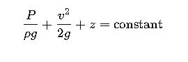
Where:
- P = pressure (Pa)
- ρ = fluid density (kg/m³)
- g = gravitational acceleration (9.81 m/s²)
- v = velocity (m/s)
- z = elevation head (m)
This equation represents the conservation of energy along a streamline.
2. Darcy–Weisbach Pressure Loss
The primary formula for pressure drop in pipelines:
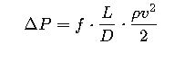
Where:
- ΔP = pressure loss (Pa)
- f = Darcy friction factor (dimensionless)
- L = pipe length (m)
- D = pipe diameter (m)
- ρ = density (kg/m³)
- v = velocity (m/s)
3. Reynolds Number (Flow Regime Indicator)
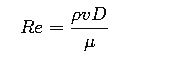
Where:
- μ = dynamic viscosity (Pa·s)
- Re < 2000 → Laminar flow
- 2000 < Re < 4000 → Transitional flow
- Re > 4000 → Turbulent flow
4. Friction Factor (Swamee–Jain Correlation for Turbulent Flow)
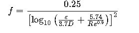
Where:
- ε = pipe roughness (m)
- D = pipe diameter (m)
- Re = Reynolds number
5. Head Loss Due to Elevation
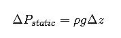
Where:
- Δz = elevation change (m)
6. Total Pressure Equation in Pipelines
The total pressure drop combines all effects:

Detailed Explanation of Variables in Pipeline Pressure Calculations
To accurately calculate pressure in pipelines, each variable must be clearly understood. Below is a breakdown of the most important variables and their typical ranges in engineering practice.
Pipe Length (L)
- Represents the total distance the fluid travels inside the pipeline.
- The longer the pipeline, the higher the pressure loss due to friction.
- Typical ranges: short industrial process lines may be only a few meters long, while transmission pipelines for oil and gas can exceed hundreds of kilometers.
Pipe Diameter (D)
- Directly affects velocity and pressure loss.
- Larger diameters reduce velocity and friction losses but increase material and installation costs.
- Common sizes: 25 millimeters for small chemical lines up to 2 meters for large water mains.
Fluid Density (ρ)
- Defines how much mass of fluid is present per unit volume.
- Higher density means higher energy requirements to move the fluid.
- For example, water has a density close to 1000 kilograms per cubic meter, while natural gas at standard conditions is less than 1 kilogram per cubic meter.
Fluid Viscosity (μ)
- Describes the internal resistance of the fluid to flow.
- Low viscosity fluids (like water) flow easily, while high viscosity fluids (like heavy oils or glycerin) generate significant pressure drops.
- Values range from less than 0.001 Pascal-seconds for gases to above 1 Pascal-second for viscous liquids.
Velocity (v)
- The speed of the fluid inside the pipe.
- Higher velocity increases friction losses exponentially.
- Typical design values: 1–2 meters per second for clean water, 10–20 meters per second for natural gas, and 0.6–1.5 meters per second for corrosive chemicals.
Roughness (ε)
- A measure of how irregular the internal pipe surface is.
- New PVC or stainless steel pipes have extremely low roughness, while old cast iron or concrete pipes may have significant roughness leading to high energy losses.
- This parameter is critical in turbulent flow calculations.
Elevation Cha nge (Δz)
- Represents the vertical difference between inlet and outlet.
- If a pipeline must pump liquid uphill, pressure must overcome gravitational forces. Conversely, downhill flow may increase velocity and risk cavitation.
- In water distribution networks, elevation change can dominate frictional losses.
Fittings and Valves (K-Factors)
- Every bend, tee, valve, or reducer contributes to additional losses.
- Engineers assign dimensionless coefficients to each fitting.
- For instance, a sharp 90-degree elbow may have a coefficient of 0.9, while a fully open gate valve may be as low as 0.15.
Real-World Applications of Pipeline Pressure Calculations
Now let’s explore two detailed case studies to show how engineers apply these variables in practice.
Case Study 1: Water Distribution Pipeline in a Municipal System
Scenario:
A city water utility needs to transport potable water from a treatment plant to a residential area located 15 kilometers away. The pipeline diameter is 300 millimeters, made of ductile iron, and includes several fittings such as elbows, gate valves, and reducers. The terrain rises by 30 meters between the source and the delivery point.
Engineering Considerations:
- Fluid properties: water at 20°C with density near 1000 kilograms per cubic meter and viscosity of approximately 0.001 Pascal-seconds.
- Design velocity: targeted between 1.2 and 2 meters per second to avoid excessive energy costs and water hammer.
- Pipe roughness: ductile iron roughness of about 0.26 millimeters.
- Elevation head: 30 meters of additional head must be overcome.
Calculation Outcome:
- Frictional losses across 15 kilometers dominate the pressure requirements.
- Fitting losses add an extra 10–15% to the total pressure drop.
- The required pump must provide sufficient pressure to cover both friction and elevation.
Result in Practice:
Engineers select a pump capable of delivering approximately 5–6 bars of pressure at the required flow rate. This ensures continuous water supply with reserve margin for peak demand and minor future expansions.
Case Study 2: Natural Gas Transmission Pipeline
Scenario:
A gas company operates a 100-kilometer high-pressure pipeline transporting natural gas from a processing facility to a city. The pipeline is made of carbon steel with a diameter of 600 millimeters. Operating pressure is maintained around 60 bar at the inlet.
Engineering Considerations:
- Fluid properties: natural gas with density close to 0.8 kilograms per cubic meter at standard conditions, adjusted for high pressure and temperature.
- Design velocity: 15 meters per second to balance efficiency and noise control.
- Pipe roughness: carbon steel new pipe with roughness of 0.045 millimeters.
- Compressibility: gas behavior deviates from ideal fluid equations, requiring correction factors.
Calculation Outcome:
- Frictional losses across 100 kilometers are substantial, even with a large diameter.
- Compressibility effects become significant, requiring advanced gas equations rather than simple liquid equations.
- Booster compressor stations are strategically placed along the route to maintain pressure within safe and efficient ranges.
Result in Practice:
The pipeline design ensures safe delivery of natural gas while minimizing compression costs. Failure to account for pressure losses would result in under-pressurized delivery and possible operational shutdowns.
Practical Notes and Industry Standards
- International Standards:
Engineers follow guidelines such as ASME B31.4 for liquid pipelines, ASME B31.8 for gas pipelines, and ISO 13623 for offshore pipelines. - Safety Margins:
Pipelines are designed with a margin above calculated pressures to ensure durability under fluctuating conditions. - Energy Efficiency:
Reducing pressure drop saves pumping or compression energy, leading to lower operational costs. - Material Selection:
Pipe material must match fluid type, temperature, and expected lifetime. For corrosive fluids, stainless steel or specialized coatings are preferred. - Digital Tools:
Engineers now use software like AFT Fathom, PipeFlow Expert, and Aspen HYSYS to simulate pressure drop with high accuracy, including transient events such as surge and water hammer.