S parameters to impedance conversion requires precise reference plane alignment and consistent characteristic impedance management.
This article details calculators, formulas, workflows, examples, normative references, and practical tips for engineers today.
S-Parameters to Impedance — Complex Reflection to Load Impedance Calculator
Why S-Parameters to Impedance Conversion Is Essential for Microwave Design
Modern RF and microwave engineering relies on scattering parameters (S-parameters) measured on network analyzers referenced to a system impedance Z0. To predict circuit behavior, design matching networks, and ensure stability, engineers convert S-parameters into impedance (Z) or admittance (Y) representations. A reliable S-parameters to impedance calculator must implement correct matrix algebra, handle complex arithmetic, and support arbitrary reference impedances and terminations.
Key functional requirements for a best-in-class calculator
- Support for single-port and multiport conversions (1-port to complex impedance, 2-port S→Z matrix transformation).
- Accurate complex arithmetic with phase-aware inputs (dB & degrees or linear complex format).
- Arbitrary reference impedance Z0 (typically 50 Ω, but also 75 Ω and others).
- Termination options (open, short, matched, arbitrary complex load) to compute input impedance under realistic loading.
- Validation checks for numerical stability (check determinants and near-singular matrices).
- Clear reporting of units, rounding rules, and calculation assumptions.
Theoretical basis and conversion formulas
Core theory: for N-port networks described by S-parameters referenced to Z0, the impedance matrix Z is given by a bilinear transform. For a 2-port network this is implemented using matrix algebra to convert S to Z.
General matrix formula (N-port)
Explanation of variables and typical values:
- Z: impedance matrix (Ω).
- Z0: characteristic/reference impedance (Ω). Typical values: 50, 75.
- I: identity matrix of size N.
- S: scattering parameter matrix (N×N) with complex entries Sij.
- (I − S)^{-1}: matrix inverse of (I − S); numerical inversion must check determinant magnitude to avoid division by near-zero.
Explicit two-port element formulas
For a 2×2 S matrix with elements S11, S12, S21, S22 and reference impedance Z0, define
Then the Z-parameters are:
Each Sij is complex: Sij = |Sij|∠θij or Sij = a + jb. Typical Z0 = 50 Ω.
Computing input impedance with termination
If port 2 is terminated with load ZL, the input impedance seen at port 1 is
Variables:
- Zin: input impedance at port 1 (Ω).
- ZL: load impedance connected at port 2 (Ω), can be complex.
- Zij: elements obtained from S→Z conversion above.
Practical calculator features and numerical safeguards
Handling special cases
- If |det(I − S)| is very small, provide a warning and use higher-precision arithmetic or perturbation methods.
- Allow inputs in dB/deg and linear complex formats; always convert to complex linear before algebra.
- Support conversions for non-50 Ω reference impedances via substitution of Z0.
- Return both magnitude/angle and rectangular complex form for transparency.
Validation and error messages
- Warn when VSWR is infinite (|Γ| = 1) or near unity (|Γ| ≈ 1) because Zin may be purely reactive or numerically unstable.
- Flag passive but non-physical S-parameter sets (violations of energy conservation or reciprocity) with references to measurement errors.
| S11 (dB) | |Γ| (linear) | VSWR | Interpretation |
|---|---|---|---|
| 0 | 1.000 | ∞ | Open or short depending on phase; total reflection |
| -1 | 0.891 | 17.9 | Very poor match |
| -3 | 0.707 | 5.83 | Significant reflection |
| -6 | 0.501 | 3.02 | Moderate mismatch |
| -10 | 0.316 | 1.93 | Common acceptable match in many systems |
| -15 | 0.178 | 1.44 | Good match |
| -20 | 0.100 | 1.22 | Very good match |
| -30 | 0.032 | 1.07 | Excellent match |
| -40 | 0.010 | 1.02 | Near perfect match |
| Component | S11 (dB / angle) | S21 (dB / angle) | S12 (dB) | S22 (dB / angle) | Reference Z0 |
|---|---|---|---|---|---|
| Small-signal amplifier | -10 dB / -30° | 18 dB / 0° | -40 dB | -10 dB / 10° | 50 Ω |
| Power amplifier (loaded) | -8 dB / -45° | 30 dB / 0° | -20 dB | -6 dB / 30° | 50 Ω |
| Directional coupler (through) | -25 dB | -0.5 dB | -20 dB | -25 dB | 50 Ω |
| 10 dB attenuator | -20 dB | -10 dB | -10 dB | -20 dB | 50 Ω |
| Connector (good) | -30 dB | -0.1 dB | -0.1 dB | -30 dB | 50 Ω |
| Directional coupler (coupled) | -25 dB | -0.5 dB | -20 dB / 90° | -25 dB | 50 Ω |
Formula walkthroughs and variable explanations
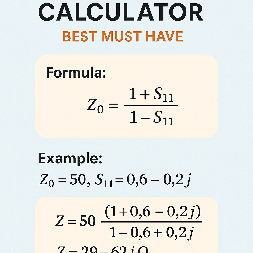
Single-port conversion from S11 to input impedance
For a single port referenced to Z0, the reflection coefficient Γ is S11. The input impedance Zin is computed by the Möbius transform:
Variable explanations and typical values:
- Γ: complex reflection coefficient, range |Γ| ≤ 1 for passive networks.
- Z0: reference impedance, common values 50 Ω and 75 Ω.
- Zin: resulting complex impedance (R + jX) in ohms.
Example variables typical ranges
- Antenna S11 at resonance: S11 ≤ −10 dB magnitude roughly |Γ| ≤ 0.316.
- High gain amplifier S21: typically +10 dB to +30 dB depending on amplifier class.
- S12 (reverse isolation) often −10 dB to −50 dB; in ideal isolators it is very low.
Worked examples — step-by-step conversions
Example 1 — Single-port S11 to complex impedance (realistic measurement)
Problem statement: A DUT measured S11 = −10 dB at 2.0 GHz with phase −60° on a 50 Ω system. Compute Zin in rectangular form.
Step 1: Convert dB to linear magnitude
Step 2: Convert polar to rectangular form
Step 3: Compute (1 + Γ) and (1 − Γ)
Step 4: Compute ratio (1 + Γ) / (1 − Γ)
Use complex division: Let numerator a + jb = 1.1580 − j0.2739 and denominator c + jd = 0.8420 + j0.2739.
Result interpretation: The DUT has a moderately resistive input with capacitive reactance (negative imaginary part) at 2 GHz for the measured reflection.
Example 2 — Two-port S-parameters to input impedance with a port termination
- S11 = 0.10
- S12 = 0.01
- S21 = 2.00
- S22 = 0.10
Compute Z-parameters and input impedance when port 2 is terminated with ZL = 50 Ω.
Step 1: Compute ΔS
Step 2: Compute Z11
Z11 = 50 × (0.99 + 0.02) / 0.79 = 50 × 1.01 / 0.79 = 50 × 1.27848 = 63.924 Ω
Step 3: Compute Z12 and Z21
Step 4: Compute Z22
Result interpretation: The two-port network yields an input impedance approximately 61.1 Ω when port 2 is terminated in 50 Ω, predominantly resistive in this simplified case.
Implementation notes for a robust calculator
Input formatting and user experience
- Allow inputs in dB/deg, real+jimag, or magnitude/angle. Normalize automatically to complex linear form before calculations.
- Provide live diagnostics: check |Γ|, VSWR, and det(I − S) and display warnings if any exceed thresholds.
- Offer optional precision control (double precision vs extended precision) for near-singular matrices.
- Give users the option to compute Z for multiple frequencies (batch mode) and export CSV or Touchstone-compatible results.
Numerical stability and best practices
- Always compute matrix inverses by LU decomposition or robust linear algebra libraries to avoid direct determinant-based inversion when possible.
- When |det(I − S)| < 1e−6, notify the user and suggest small regularization or offsetting reference plane if measurement error suspected.
- Provide unit tests covering extremes: perfect match, open/short (|Γ| = 1), and high gain unstable amplifiers.
Standards, references, and further reading
Authoritative references and application notes that underpin correct S→Z conversion and best practices include:
- David M. Pozar, "Microwave Engineering", 4th Edition — canonical textbook for scattering-parameter theory and network conversions.
- National Instruments, "S-Parameter Basics" — practical primer on S-parameters and measurement considerations: https://www.ni.com/en-us/innovations/white-papers/06/s-parameter-basics.html
- Keysight Technologies application notes and technical resources on S-parameter measurement and de-embedding: https://www.keysight.com
- NIST technical resources on calibration and network analyzer traceability: https://www.nist.gov
- IEEE Xplore papers on network parameter conversions and measurement uncertainty (search for S-parameter calibration and de-embedding): https://ieeexplore.ieee.org
Standards and recommended practices
- Follow established network analyzer calibration procedures (SOLT, TRL) to ensure S-parameter accuracy before conversion.
- For connector and cable specifications, consult IEC and manufacturer datasheets (e.g., IEC 61169 series).
- When working with power amplifiers, consult IEEE standards on measurement of RF amplifier parameters for safe and consistent procedures.
Checklist for deploying an S-parameters to impedance calculator
- Accept flexible input formats and clarify the reference impedance.
- Implement robust complex arithmetic and matrix inversion routines.
- Provide clear warnings for ill-conditioned inputs and numerical instability.
- Include batch processing and export capabilities for frequency sweeps.
- Document assumptions: plane of reference, calibration state, and units.
Security and verification
- Validate uploaded Touchstone files and sanitize inputs to prevent malformed data from breaking calculations.
- Include verification tests: convert S→Z→S and check consistency within numerical tolerance.
Summary of recommended "must-have" features for the best calculator
- Accurate S→Z matrix transform with robust numerical methods.
- Support for arbitrary Z0 and complex terminations.
- Full support for single-port and multiport networks with clear diagnostics.
- Exportable results, batch frequency handling, and measurement-related checks.
- Authoritative documentation and links to standards and application notes.
Implementing the above ensures that a professional-grade S-parameters to impedance calculator serves both design verification and measurement analysis tasks, reduces conversion errors, and supports reliable RF system engineering workflows.
For further technical detail, consult Pozar's textbook and the cited application notes from measurement-equipment vendors and national laboratories listed above. Keep measurement uncertainty and calibration front-and-center when interpreting conversions in practice.