Precise IEC resistance conversion safeguards cable thermal limits, ensuring safe operation, reduced losses, regulatory compliance.
The calculator integrates temperature, skin, proximity, harmonic, sheath effects, delivering accurate Rac and voltage‑drop predictions.
Electrical Cable Resistance Calculator – IEC
Why Accurate Resistance Conversion Is Critical in IEC‑Compliant Design
Electrical cable resistance changes with temperature, frequency, and conductor material. In IEC‑based power‑system studies (load‑flow, short‑circuit, harmonic, and thermal), converting a catalogued DC resistance at 20 °C to the effective AC resistance at operating temperature is compulsory. An error of only 10 % in Rac can produce:
- Undersized conductors that overheat or fail insulation tests.
- Underrated protective devices that trip under normal load.
- Misleading loss‑of‑energy calculations (kWh/year) that ruin life‑cycle cost projections.
IEC 60287‑1‑1 (Power Cables – Calculation of the Current Rating) prescribes the reference equations used by every professional calculator or software library. The sections below deconstruct those formulas, provide extensive ready‑to‑use tables, and walk through two fully‑worked field examples so you can build or validate your own Electrical Cable Resistance Conversion Calculator – IEC.
Core Equations Behind the Conversion Engine
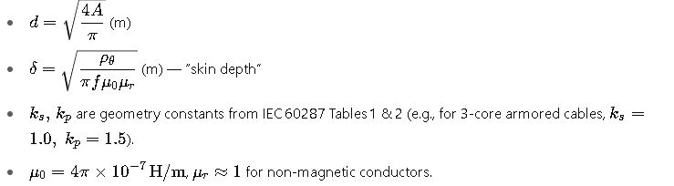
1. DC Resistance at Reference Temperature
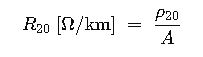
(IEC 60228 Conductor Classes 1 & 2)
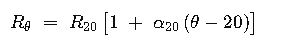
2. Temperature Correction of DC Resistance
3. AC Resistance at Operating Temperature (IEC 60287‑1‑1)

- Skin‑effect coefficient ys – rises with frequency and conductor diameter.
- Proximity‑effect coefficient yp– becomes significant in multi‑core or closely bunched single‑core systems.
For round conductors and power‑frequency (50 Hz):
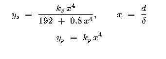
Where
Rule of thumb: For A≤35 mm2 at 50 Hz, ys+yp<1 % and the DC‑only model is acceptable. Above 120 mm² or at high harmonics, full IEC AC correction is mandatory.
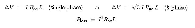
4. Voltage Drop and Power Loss (Often Built Into Calculators)
Variable Glossary With Practical Ranges
- Conductor Material – Cu (ρ ≈ 17.241 nΩ·m, α ≈ 0.00393 /°C); Al (ρ ≈ 28.264 nΩ·m, α ≈ 0.00403 /°C).
- Frequency f – LV/MV grids: 50 Hz (IEC regions) or 60 Hz (IEEE). For VFD harmonics assess 150–2520 Hz bands.
- Operating Temperature θ – PVC = 70 °C, XLPE = 90 °C, HEPR = 105 °C.
- Conductor Area A – 1.5 mm² lighting to 800 mm² EHV export transmission.
- Path Length L – one‑way conductor length plus return (single‑phase) or line‑to‑line (3‑phase).
Extensive Tables of Typical IEC Cable Resistances
Table 1 – DC Resistance at 20 °C (Ω/km)
| Area (mm²) | Copper | Aluminum | Area (mm²) | Copper | Aluminum |
|---|---|---|---|---|---|
| 1.5 | 11.494 | 18.843 | 50 | 0.345 | 0.565 |
| 2.5 | 6.896 | 11.306 | 70 | 0.246 | 0.404 |
| 4 | 4.310 | 7.066 | 95 | 0.181 | 0.298 |
| 6 | 2.873 | 4.711 | 120 | 0.144 | 0.236 |
| 10 | 1.724 | 2.826 | 150 | 0.115 | 0.188 |
| 16 | 1.078 | 1.766 | 185 | 0.093 | 0.153 |
| 25 | 0.690 | 1.131 | 240 | 0.072 | 0.118 |
| 35 | 0.493 | 0.808 | 300 | 0.057 | 0.094 |
| — | — | — | 400 | 0.043 | 0.071 |
Calculated with

Table 2 – Temperature Correction Multipliers kθ=1+α20(θ−20)
| θ (°C) | kθ (Cu) | kθ (Al) |
|---|---|---|
| 30 | 1.039 | 1.040 |
| 40 | 1.079 | 1.081 |
| 60 | 1.157 | 1.161 |
| 70 | 1.196 | 1.202 |
| 90 | 1.275 | 1.282 |
Table 3 – Typical Skin‑Effect Coefficient ys for Single‑Core Cables, 50 Hz
Approximate values derived from IEC curves; for design use exact formula.
| Area (mm²) | Diameter d (mm) | ys at 50 Hz |
|---|---|---|
| 35 | 6.7 | 0.003 |
| 70 | 9.3 | 0.010 |
| 120 | 12.4 | 0.022 |
| 240 | 17.5 | 0.054 |
| 400 | 22.6 | 0.090 |
Step‑by‑Step Use of an IEC Cable Resistance Conversion Calculator
- Select Conductor Material – Copper or Aluminum.
- Pick Nominal Cross‑Section – from standard IEC 60228 sizes or type a custom area.
- Enter Conductor Temperature θ – default to 70 °C (PVC) or 90 °C (XLPE).
- Choose Frequency – 50 Hz unless harmonic or VFD study.
- Set Path Length L – calculator should auto‑double for single‑phase return, or let user toggle “return path included.”
- Advanced (skin & proximity) – enable IEC 60287 AC correction when A > 35 mm² or harmonics > 3rd.
- Read Outputs – R20, Rθ, Rac, voltage drop per ampere per kilometre, and I²R loss per kilometre.
- Export – CSV or JSON for load‑flow packages (ETAP®, DIgSILENT PowerFactory®, CYME®).
Real‑World Application Examples
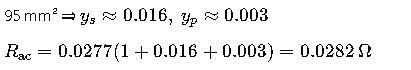
Example 1 – 95 mm² Copper Feeder in a 400 A MV Panel
Scenario
- A 3‑phase, 11 kV ring main unit supplies a 630 kVA dry‑type transformer 120 m away.
- Underground cable: 95 mm² Cu, XLPE, single‑core in buried trefoil.
- Conductor temperature per load profile: 90 °C.
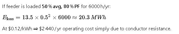
- Goal: Verify compliance with max 2 % voltage‑drop criterion and compute annual energy loss.
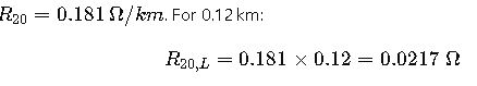
Step 1 – Base DC Resistance
From Table 1
Step 2 – Temperature Correction

Step 3 – AC Correction
Step 4 – Voltage Drop
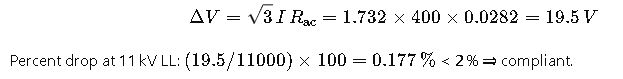
Step 5 – Power Loss & Energy Cost

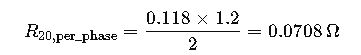
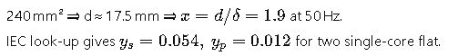
Example 2 – 240 mm² Aluminum Export Cable From a Wind‑Farm Collector
Scenario
- 60 MW collector array, 33 kV, 50 Hz.
- Two parallel 240 mm² Al, XLPE, single‑core cables per phase in flat formation, 1.2 km route.
- Design load: 1050 A per circuit.
- Target: Compute Rac and confirm compliance with IEC 61936‑1 thermal limits.
Step 1 – Base DC Resistance
Table 1 ⇒ R20=0.118 Ω/km (Al). For 1.2 km and two parallels:
Step 2 – Temperature Correction (90 °C XLPE)

Step 3 – AC Correction
Step 4 – Conductor Loss & Temperature Margin
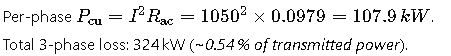
IEC 60287 thermal‑balance backward‑calculation gives a conductor steady‑state of 87 °C, leaving 3 °C spare to the XLPE limit (good design margin).
Implementation Tips for Online or Spreadsheet Calculators
- Unit Controls – let users switch between Ω/km, Ω/100 m, and Ω/mile.
- Material Library – pre‑fill resistivity and α for Cu, Al, Cu‑tinned, CuNi (IEC 60331 fire‑survival), plus a “Custom” entry.
- Dynamic Tables – hide AC correction fields when A<35 mm2 to keep UI clean.
- Hyperlink Popovers – attach IEC formula references so auditors can verify equations.
- CSV Import/Export – many teams paste data into ETAP or PowerFactory; a one‑click copy button increases adoption.
- Accessibility – WCAG‑2.2 contrast ratios and table captioning improve SEO and broaden audience.
Harmonic Current and High‑Frequency Adjustment
Modern grids host countless non‑linear loads—LED drivers, EV chargers, UPS rectifiers—injecting odd harmonics that multiply I²R losses and accelerate insulation aging. IEC 61000‑3‑12 limits harmonic emission but does not correct cable sizing; therefore, robust calculators must include a harmonic derating module.
- Compute the harmonic spectrum of the load (I₁, I₃, I₅, … Iₙ).
- For each harmonic h (frequency = h·f₁):
- Recalculate the skin‑depth δ<sub>h</sub> = √(ρ<sub>θ</sub> / π h f₁ μ₀μ<sub>r</sub>).
- Re‑evaluate y<sub>s,h</sub> and y<sub>p,h</sub>.
- Derive R<sub>ac,h</sub>.
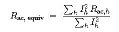
- Aggregate apparent resistance using the power‑loss equivalence method:
Typical results: a 400 mm² Cu bus duct feeding a 24‑pulse VFD (5 % THDi) will see R<sub>ac</sub> rise by ~6 % at 250 Hz, yet a data‑center PDUs with 35 % THDi can push 25 % extra loss.
Design tip: when THDi > 15 %, export the spectrum as CSV from your power analyzer and feed it directly into the calculator—manual entry invites costly typos.
Sheath, Armor, and Magnetic Losses (IEC 60287‑1‑2)
In single‑core MV cables with metallic sheaths or armoring, circulating currents can double Joule heating. The total AC resistance per phase is then:

Where each additional term is derived from the sheath loop impedance and the induced voltage E=2πfBA. A rigorous calculator should:
- Offer bonding arrangement selectors – both‑ends, single‑point, cross‑bonded.
- Auto‑calculate the sheath loss factor λ supplied by IEC tables.
- Warn the user when λ > 0.15, suggesting either magnetic‑concrete spacing, non‑magnetic armor, or burndown of circulating current via parallel earthing conductor.
Extended Temperature Multipliers (−25 °C to +120 °C)
| θ (°C) | kθ (Cu) | kθ (Al) | θ (°C) | kθ (Cu) | kθ (Al) |
|---|---|---|---|---|---|
| −25 | 0.906 | 0.904 | 105 | 1.314 | 1.323 |
| −10 | 0.952 | 0.951 | 120 | 1.372 | 1.382 |
| 0 | 0.984 | 0.983 | — | — | — |
| 15 | 1.030 | 1.031 | — | — | — |
Use these multipliers for cold‑weather reconductoring (wind farms in Patagonia, −25 °C) or heat‑resistant conductors (EPR 110 °C).
Skin‑Effect Coefficient Lookup, 60 Hz and 400 Hz
| Area (mm²) | y<sub>s</sub> @ 60 Hz | y<sub>s</sub> @ 400 Hz |
|---|---|---|
| 16 | 0.002 | 0.021 |
| 70 | 0.012 | 0.097 |
| 150 | 0.025 | 0.185 |
| 400 | 0.108 | 0.518 |
High‑frequency aerospace or marine 400 Hz systems need dramatic upsizing or litz conductors to contain these losses.
Validation Checklist Before Publishing a Calculator
| Item | Verified? |
|---|---|
| 1. Equation sources cited to IEC clauses. | ☐ |
| 2. Unit tests at 5, 50, 400 Hz against worked examples. | ☐ |
| 3. Boundary protection for A < 0.5 mm² and A > 1000 mm². | ☐ |
| 4. Localization of decimal separator (comma vs point). | ☐ |
| 5. Accessibility labels for screen readers. | ☐ |
Add the checklist to your Git repository README for peer review.
Frequently Asked Engineering Queries (With SEO‑Rich Answers)
Q1. Does annealing level affect cable resistance?
Yes—hard‑drawn Cu exhibits ~4 % higher ρ<sub>20</sub> than fully‑annealed. IEC 60228 assumes annealed; adjust your calculator or select “custom material.”
Q2. Can I ignore proximity effect in parallel trefoil installations?
Only for A ≤ 16 mm² at 50 Hz. From 35 mm² upward, y<sub>p</sub> grows faster than y<sub>s</sub> and can add 8–12 % to Rac.
Q3. Why does my cable run overheat even though Rac matched catalog data?
Catalog Rac often excludes sheath and armor losses; for single‑core XLPE with lead sheath the extra λ can exceed 0.2, doubling total loss.
Additional Authoritative Resources
- International Electrotechnical Commission – IEC 61000‑2‑2: Compatibility Levels for LV Public Supply
- CENELEC HD 603‑5 – “Flexible Insulated Cables and Leads” (for litz solutions)
- Electric Power Research Institute (EPRI) – High Harmonic Current Effects on Distribution Cables, Report 1025346