Total Dissolved Solids (TDS) is a critical parameter for assessing water quality in diverse industrial, municipal, and environmental applications worldwide. Measuring and calculating TDS reveals concentrations of inorganic salts, organic matter, and ions influencing taste, health, agriculture, and equipment.
TDS (Total Dissolved Solids) Calculator — µS/cm & mS/cm → ppm
Quickly convert conductivity to TDS using a selectable conversion factor. Valid for water testing, aquariums, hydroponics, and labs.
How is TDS estimated from conductivity?
Why different factors (0.5–0.7)?
Formulas used
If input is in mS/cm: TDS(ppm) = EC(mS/cm) × 1000 × k.
Extended Reference Table of Common TDS Conversion Factors
TDS is often calculated from electrical conductivity (EC) using a conversion factor (f). This factor varies depending on the ionic composition of the water, typically ranging from 0.5 to 0.9. The following table shows common values used in engineering practice, laboratory analysis, and regulatory compliance.
Table 1. Common Conversion Factors for TDS Calculation
| Water Type / Condition | Conductivity Range (µS/cm) | Conversion Factor (f) | Approx. TDS (ppm) = EC × f |
|---|---|---|---|
| Distilled Water | 0 – 2 | 0.55 | Near 0 ppm |
| Rainwater (clean) | 10 – 50 | 0.55 – 0.6 | 5 – 30 ppm |
| Surface Water (rivers, lakes) | 30 – 500 | 0.6 – 0.65 | 20 – 325 ppm |
| Groundwater (shallow wells) | 100 – 1500 | 0.64 – 0.67 | 64 – 1005 ppm |
| Municipal Tap Water (typical) | 200 – 800 | 0.65 | 130 – 520 ppm |
| Brackish Water | 1000 – 10,000 | 0.65 – 0.7 | 650 – 7000 ppm |
| Seawater | 40,000 – 55,000 | 0.85 – 0.9 | 34,000 – 50,000 ppm |
| Industrial Cooling Water | 200 – 1500 | 0.65 – 0.7 | 130 – 1050 ppm |
| Desalinated (RO-treated) Water | 20 – 200 | 0.5 – 0.55 | 10 – 110 ppm |
| High-Purity Boiler Feedwater (power plants) | < 20 | 0.5 | < 10 ppm |
| Wastewater (treated effluent) | 200 – 1500 | 0.65 – 0.7 | 130 – 1050 ppm |
| Agricultural Irrigation Water (FAO Guidelines) | 200 – 2000 | 0.65 | 130 – 1300 ppm |
Essential Formulas for TDS Calculation
Formula 1: Direct Gravimetric Method
The gravimetric method is the reference standard, involving evaporation and weighing:
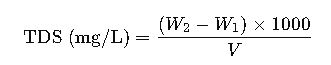
- W1= initial weight of dish (mg)
- W2= final weight of dish + residue (mg)
- V= volume of water sample evaporated (mL)
This method is highly accurate but time-consuming, used mainly in laboratory compliance testing.
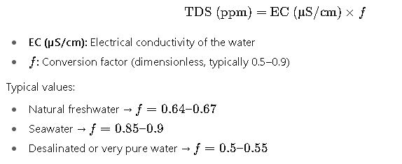
Formula 2: Conductivity Conversion Method
Most field applications use conductivity-based calculation:
Formula 3: Empirical Multi-Ion Equation
For high accuracy where ionic composition is known:
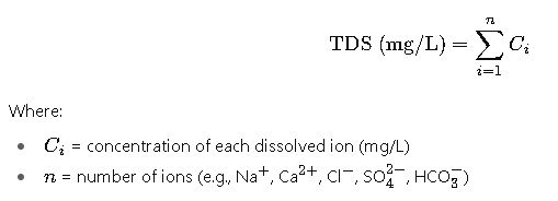
This requires ion chromatography or spectrophotometric analysis, but provides precise ion-specific results.
Formula 4: Relation with Salinity
For seawater and brackish water:
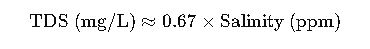
This approximation is often used in oceanography and desalination plants.
Explanation of Variables and Their Ranges
- Electrical Conductivity (EC):
- Measured in µS/cm or mS/cm at 25°C.
- Range: 0 (distilled water) to >55,000 µS/cm (seawater).
- Conversion Factor (f):
- Dimensionless, based on ionic composition.
- Range: 0.5–0.9.
- Volume (V):
- Sample size for gravimetric method, usually 100–250 mL.
- Residue Weight Difference (W2 – W1):
- Mass of dissolved solids after evaporation.
- Can be as low as 1 mg in ultrapure water tests.
Practical Examples of TDS Calculation
Example 1: Calculation for Municipal Tap Water
Given data:
- EC = 650 µS/cm
- Conversion factor f=0.65
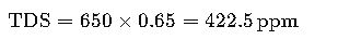
Interpretation:
This water falls within the acceptable range for WHO drinking water (<1000 ppm).
Example 2: Calculation for Brackish Groundwater
Given data:
- EC = 3500 µS/cm
- f=0.67
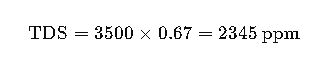
Interpretation:
This water exceeds WHO drinking standards but can be used for irrigation with restrictions (FAO guidelines recommend <2000 ppm for most crops).
Real-World Case Studies
Case Study 1: Desalination Plant Performance Monitoring
Background:
A coastal desalination plant producing potable water needs to verify RO system efficiency. The feedwater is seawater with EC = 52,000 µS/cm. After treatment, the permeate is tested.
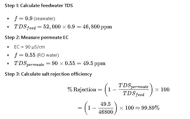
Result:
The RO system is operating within design limits (>99% rejection).
Case Study 2: Irrigation Water Suitability for Agriculture
Background:
An agricultural cooperative wants to evaluate groundwater for irrigation.
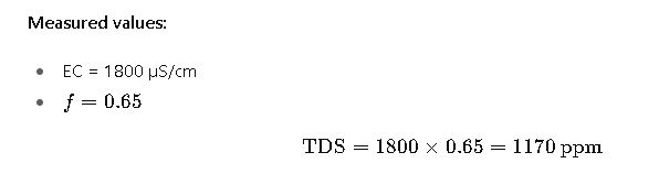
Interpretation:
- According to FAO standards:
- <700 ppm → Excellent water quality
- 700–2000 ppm → Permissible for most crops with some restrictions
- 2000 ppm → Unsuitable without treatment
Conclusion:
The water (1170 ppm) is acceptable for irrigation of moderately salt-tolerant crops (e.g., barley, cotton, sugar beet), but could negatively affect sensitive crops like beans and citrus.
Importance of Temperature Compensation
EC measurements must be corrected to 25°C reference:
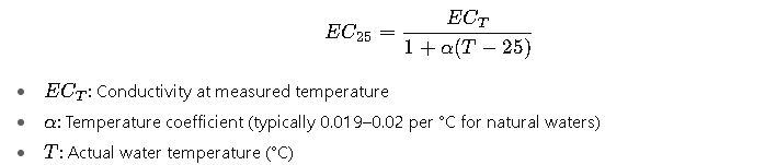
Failure to compensate temperature can lead to errors of 2% per °C, severely impacting TDS estimates.
Standards and Guidelines
- WHO Drinking Water Guidelines: TDS < 1000 ppm recommended for palatability (WHO source).
- US EPA Secondary Drinking Water Regulations: TDS < 500 ppm is optimal (EPA source).
- FAO Irrigation Water Standards: 700–2000 ppm permissible depending on crop tolerance (FAO source).