This article defines cable reactance calculation requirements for IEC-compliant tools and practical applications worldwide today.
Engineers require an affordable, accurate cable reactance calculator integrating IEC standards and installation parameters efficiently.
Cable Reactance Calculator — IEC-compatible, affordable field tool
Technical background: reactance, inductance and IEC relevance
Cable reactance is the frequency-dependent imaginary part of series impedance. It arises from magnetic flux linkage and conductor geometry, and it governs voltage drop, short-circuit impedance and system stability. Accurate reactance calculation is mandatory for protective device coordination, fault calculations and compliance with IEC mandates for distribution and transmission installations.IEC normative documents reference methods to compute cable and overhead conductor impedances using geometric mean radii (GMR), mutual distances (GMD / Deq) and material constants. A compact, affordable IEC tool must implement those equations, support typical conductor data sets, and allow parametric sensitivity analysis for engineers and planners.Core formulas and variable definitions
All formulas below use SI units. Frequency f in hertz (Hz), lengths in meters (m), radii in meters (m), inductance L in henry per metre (H/m) and reactance X in ohm per metre (Ω/m) or ohm per kilometre (Ω/km).
Fundamental electromagnetic relations
Inductance per unit length for conductors arranged so that an equivalent spacing Deq and GMR r' represent geometry:
L' = 2 × 10⁻⁷ × ln(Deq / r') H/m
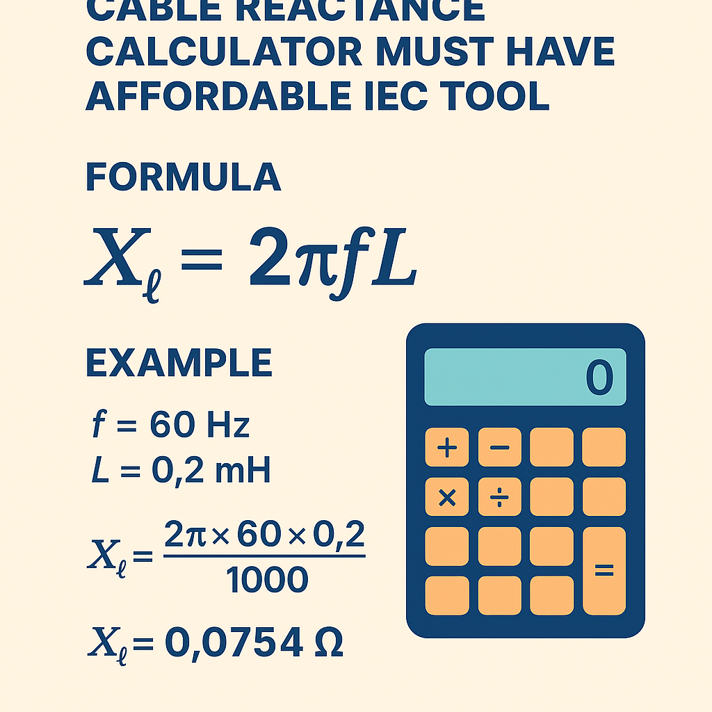
Reactance per unit length (angular relation):
Reactance per kilometre (practical reporting):
X (Ω/km) = 1.25663706 × 10⁻³ × f × ln(Deq / r')
Variable explanations and typical ranges
- f — frequency, typical values: 50 Hz (Europe, Africa, Asia), 60 Hz (Americas, parts of Asia).
- Deq — equivalent spacing (m). For three-phase overhead equilateral spacing, Deq equals phase-to-phase centre distance (typical 0.3–1.0 m). For trefoil cable cores Deq is centre-to-centre core spacing (typical 0.02–0.05 m).
- r' — geometric mean radius (GMR) in metres. For solid circular conductor r' = r × e-1/4 where r is geometric radius (m). Typical r' values depend on conductor cross-section (see tables).
- ln(Deq / r') — natural logarithm of the ratio, dimensionless; it sets the magnitude of L' and X'.
- L' — inductance per metre, usually in range 0.2–2.0 × 10⁻⁶ H/m depending on geometry.
- X (Ω/km) — commonly expressed per kilometre; typical ranges: overhead lines 0.2–0.6 Ω/km, medium voltage cables 0.05–0.2 Ω/km depending on configuration and size.
How to compute r' (GMR) for standard conductors
For a solid circular conductor with area A (m2) and diameter d (m):
GMR (r') for a solid conductor: r' = r × e-1/4 ≈ r × 0.77880078
For stranded conductors, standards provide empirical GMR correction factors (see IEC 60228 and IEC 60287). When stranded correction tables are not available, use conductor manufacturer GMR values or apply an approximate correction factor between 0.75 and 0.82 of the outer strand radius depending on stranding.
Extensive tables: reactance per km for common conductor sizes and configurations
Tables below present computed reactance values using the formula X (Ω/km) = 1.25663706 × 10⁻³ × f × ln(Deq / r'). Conductor cross-sections selected: 16, 35, 70, 95, 120, 240, 400 mm2. Diameter approximations assume circular equivalent copper conductors with area A = cross-section. Values are representative; actual stranded GMR and insulation geometry alter results. Results shown for f = 50 Hz and for three Deq ranges typical for overhead lines.
| Conductor (mm²) | Approx r' (m) | X (Ω/km) @50Hz, Deq=0.3 m | X (Ω/km) @50Hz, Deq=0.4 m | X (Ω/km) @50Hz, Deq=1.0 m |
|---|---|---|---|---|
| 16 | 0.001758 | 0.323 | 0.341 | 0.399 |
| 35 | 0.002599 | 0.299 | 0.317 | 0.374 |
| 70 | 0.003676 | 0.276 | 0.295 | 0.352 |
| 95 | 0.004285 | 0.267 | 0.285 | 0.343 |
| 120 | 0.004815 | 0.260 | 0.278 | 0.335 |
| 240 | 0.006808 | 0.238 | 0.256 | 0.314 |
| 400 | 0.008787 | 0.222 | 0.240 | 0.298 |
For underground cables in trefoil and for single-core in ducts the Deq values are much smaller. The table below shows typical cable reactances at 50 Hz for compact configurations.
| Conductor (mm²) | Approx r' (m) | X (Ω/km) @50Hz, Deq=0.02 m | X (Ω/km) @50Hz, Deq=0.03 m | X (Ω/km) @50Hz, Deq=0.05 m |
|---|---|---|---|---|
| 16 | 0.001758 | 0.153 | 0.178 | 0.210 |
| 35 | 0.002599 | 0.128 | 0.154 | 0.186 |
| 70 | 0.003676 | 0.106 | 0.132 | 0.164 |
| 95 | 0.004285 | 0.097 | 0.122 | 0.154 |
| 120 | 0.004815 | 0.089 | 0.115 | 0.147 |
| 240 | 0.006808 | 0.068 | 0.093 | 0.125 |
| 400 | 0.008787 | 0.052 | 0.077 | 0.109 |
Design implications and common use-cases for an affordable IEC tool
An effective cable reactance calculator targeted at engineers and planners must include:- Built-in conductor library: common IEC conductor sizes, manufacturer GMRs and DC resistances (at 20 °C).
- Geometry models: overhead (phase spacing), trefoil, single-core in duct, flat formation, and sectoral arrangements.
- Frequency selection for 50 Hz or 60 Hz and harmonic frequency input for high-frequency studies.
- Automatic unit conversion and reporting in Ω/km, mΩ/m, and %Z at rated voltage.
- Options for sheath bonding, screen effects and proximity factors (simplified or advanced models).
- Exportable tables and reports for project documentation and IEC compliance evidence.
Practical examples: full development and detailed solutions
Case study 1 — Overhead three-phase line, fault reactance estimate (95 mm² copper)
Problem statement: A three-phase overhead distribution line uses 95 mm² copper conductors, arranged in an equilateral triangle with phase-to-phase centre spacing Deq = 0.30 m. Frequency is 50 Hz. Determine:- Reactance per km (Ω/km).
- Total series reactance for 12 km span.
- Typical single-phase short-circuit current magnitude at the receiving end if the substation source behind the line has Thevenin reactance equal to 0.5 Ω and nominal voltage is 11 kV line-to-line.
- Conductor: 95 mm² copper.
- From the GMR table above: r' ≈ 0.004285 m.
- Deq = 0.30 m.
- Frequency f = 50 Hz.
ln(69.99) ≈ 4.248
Step 3 — reactance per km using formula:X (Ω/km) = 1.25663706 × 10⁻³ × f × ln(Deq / r')
X = 1.25663706 × 10-3 × 50 × 4.248 ≈ 0.2669 Ω/km
Step 4 — total reactance of 12 km line:Case study 2 — Underground trefoil cable feeder voltage drop (240 mm² copper)
Problem statement: A 240 mm² copper trefoil cable feeds a distribution load 1.2 km away. The cores are arranged with Deq ≈ 0.03 m (typical trefoil). Frequency 50 Hz. The balanced load current is 400 A per phase at rated voltage 11 kV. Compute:- Reactance per km (Ω/km).
- Total series reactance of the feeder.
- Reactive voltage drop magnitude (line-to-line expressed as percentage of nominal line-to-line voltage).
- Conductor: 240 mm² copper; r' ≈ 0.006808 m.
- Deq = 0.03 m, f = 50 Hz, length = 1.2 km, I_load = 400 A.
ln(4.404) ≈ 1.483
Step 3 — reactance per km:X (Ω/km) = 1.25663706 × 10-3 × 50 × 1.483 ≈ 0.0932 Ω/km
Step 4 — total reactance for 1.2 km:%V_drop = (77.47 / 11,000) × 100% ≈ 0.705%.
Interpretation: Reactive voltage drop alone is small (sub-percent) for this feeder and load. For full voltage regulation assessment include resistive drop, power factor, and harmonics. Cable reactance is low because of compact geometry and large conductor size.Advanced considerations for an IEC-focused calculator
Engineers should expect the tool to address additional physical effects and provide configurable accuracy/performance trade-offs:- Skin effect and proximity effect at higher frequencies or harmonics: these increase effective series impedance; the tool should optionally include frequency-dependent impedance models (IEC 60287 models or Carson’s equations where applicable).
- Screen and sheath effects: bonded and cross-bonded configurations change positive- and zero-sequence impedance. The calculator must model bonded sheath returns and cross-bonding permutations for accuracy in fault studies.
- Temperature dependence: DC resistance varies with conductor temperature; electrolyte or insulation temperature affects impedance. Include R(T) corrections and allow user-specified operating temperatures.
- Transposition and mutual coupling: three-phase overhead lines transposed vs. untransposed influence sequence impedances; provide GMD and GMR averaging options and transposition modeling.
- Validation with manufacturer data: permit importing of vendor impedance tables and compare computed results to those data for calibration.
Validation and uncertainty analysis
A credible affordable IEC tool should:- Provide uncertainty estimates: sensitivity of X to Deq and r' should be displayed using partial derivatives or Monte Carlo sampling for uncertain geometry.
- Cross-check against reference tables: built-in quick-check comparisons against IEC/IEEE tabulated values reduce user errors.
- Include unit tests and sample projects reflecting common network topologies for regression validation.
Practical workflow for using a cable reactance calculator
Engineers typically follow these steps:- Select conductor and verify GMR (use manufacturer or IEC tables).
- Define geometry: choose overhead spacing, trefoil centres or duct positions.
- Enter frequency and temperature; select sheath bonding option.
- Compute L', X' per metre and convert to Ω/km.
- Apply results into load flow, short-circuit and protection coordination studies.
- Export results and normative compliance statements for the project dossier.
Normative references and authoritative links
The following normative documents and authoritative resources are essential to implement or validate a compliant cable reactance calculator:
- IEC 60287 series — Electric cables — Calculation of the continuous current rating (ampacity). Relevant for thermal and conductor parameters. Publisher: International Electrotechnical Commission. https://www.iec.ch/
- IEC 60228 — Conductors of insulated cables. Defines conductor classes and cross-section conventions. https://www.iec.ch/
- IEC 60909 — Short-circuit currents in three-phase AC systems. Provides methodology for fault calculations using sequence impedances. https://www.iec.ch/
- IEEE Std 80 / IEEE Std 141 — Grounding and power system design guides useful for grounding and system fault studies. https://standards.ieee.org/
- CIGRE technical brochures and working groups on cable impedance and screening effects provide practical field-validated models. https://www.cigre.org/
Implementation tips for developers and engineers
- Pre-populate conductor libraries with IEC 60228 standard areas and typical stranded conductor GMRs; allow user overrides.
- Offer geometric templates (trefoil, flat, single-core in duct) with editable parameters and real-time X preview.
- Allow batch calculations for multi-circuit networks and generate CSV or PDF reports including the calculation trace for auditability.
- Expose API endpoints to integrate the calculator into larger network analysis workflows and SCADA planning tools.
- Implement unit-aware inputs to avoid conversion mistakes (mm² vs. in², m vs. mm, km vs. m).
Validation examples and recommended test-cases
Include these scenarios in the test-suite of a tool to guarantee IEC alignment and practical robustness:
- Short overhead test: multiple Deq values (0.3, 0.6, 1.0 m) for small and large conductors; compare to hand-calculated values and tabulated references.
- Cable bundling test: compute reactance for trefoil and flat formations at close spacings (0.02–0.05 m) across conductor sizes, compare to manufacturer impedance tables.
- Temperature sweep: show R and X variation with temperature up to 90 °C and demonstrate correct R(T) correction.
- Harmonic scenario: compute series impedance at 5th and 7th harmonic frequencies and compare against frequency-dependent models to validate skin/proximity implementations.
SEO and product positioning guidance
For a product page or technical documentation that targets search demand for "Cable Reactance Calculator", position content around:- Key features: "IEC compliant", "affordable", "accurate reactance per km", "GMR/GMD calculations", "sheath bonding and proximity effects".
- Target long-tail queries: "calculate cable reactance for trefoil 240 mm2", "overhead line reactance calculator 50Hz", "how to compute cable reactance per km IEC".
- Provide downloadable worked examples and spreadsheet templates to increase engagement and backlinks from engineering blogs and standards discussions.
Summary of best practices for users
- Always validate computed r' values against manufacturer data—stranded conductors differ from solid approximations.
- Use geometry representative of installed conditions: burial depth, duct spacing and phase arrangement materially change reactance.
- For protection and fault studies include R, sequence impedances, and sheath bonding models per IEC 60909 for robust results.
- Choose an IEC-aware calculator that documents its assumptions and provides exportable calculation traces for audits.
Further reading and authoritative resources
- IEC web page (global IEC catalogue): https://www.iec.ch/ — search for IEC 60287, IEC 60228 and IEC 60909.
- IEEE Xplore standards and guides: https://standards.ieee.org/
- CIGRE technical brochures on cable system modeling: https://www.cigre.org/
- Electric power engineering handbooks and university texts on transmission line theory and cable parameters (for advanced derivations and frequency-dependent modeling).
Implementing a robust, affordable IEC-compliant cable reactance calculator requires blending rigorous electromagnetic formulas, practical conductor and geometry data, and transparent reporting to satisfy engineering and regulatory needs. The formulas and worked examples here provide a reproducible basis for both manual checks and software implementation.