Free Instant Conductor R/X Converter — Convert Ohms/1000 ft to Ohms/km with Cable Data

Free instant conductor R x converter convert ohms provides rapid resistance calculation for cable runs.

Tool outputs ohms per 1000 ft and per km using conductor size, material, and temperature.

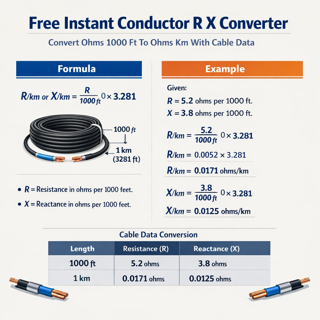
Conductor R–X Converter: Ohms per 1000 ft to Ohms per km with Cable Data

Resistance per 1000 ft (Ω/1000 ft)

Reactance per 1000 ft (Ω/1000 ft)

Advanced options

Conductor preset (optional) Custom (user-defined) ACSR 477 kcmil Hawk (60 Hz, typical) ACSR 336.4 kcmil Linnet (60 Hz, typical) Copper 500 kcmil cable (60 Hz, typical)

Parallel conductors per phase (n)

Line length to evaluate (km)

System frequency (Hz)

Upload a nameplate or line diagram photo to automatically suggest conductor and impedance values.

📷 Fill inputs from image (AI)

⚡ More electrical calculators Reiniciar Copiar Compartir

Enter resistance and/or reactance per 1000 ft to obtain the converted values in ohms per km.

🧠 Explain my result 🔍 Review my inputs

Formulas used (ohms per 1000 ft to ohms per km)

• Unit conversion factor between 1000 ft and 1 km:
  1 ft = 0.3048 m
  1 km = 1000 m = 3280.8399 ft
  So, 1 km / 1000 ft = 3280.8399 / 1000 ≈ 3.28084
• Resistance per km (single conductor):
  R_km_single [Ω/km] = R_1000ft [Ω/1000 ft] × 3.28084
• Reactance per km (single conductor):
  X_km_single [Ω/km] = X_1000ft [Ω/1000 ft] × 3.28084
• Effective per km values with n parallel conductors per phase:
  R_km_effective [Ω/km] = R_km_single / n
  X_km_effective [Ω/km] = X_km_single / n
• Total series impedance over a line length L:
  R_total [Ω] = R_km_effective [Ω/km] × L [km]
  X_total [Ω] = X_km_effective [Ω/km] × L [km]
  |Z_total| [Ω] = sqrt(R_total² + X_total²)

Typical R and X values (60 Hz, per phase)

Conductor type	R (Ω/1000 ft)	X (Ω/1000 ft)	R (Ω/km)	X (Ω/km)
ACSR 477 kcmil Hawk (overhead)	0.031	0.275	0.10	0.90
ACSR 336.4 kcmil Linnet (overhead)	0.047	0.280	0.15	0.92
Copper 500 kcmil (power cable)	0.018	0.220	0.06	0.72
Generic MV cable, 240 mm² Al	0.036	0.210	0.12	0.69

Technical FAQ for this conductor R–X converter

1. When should I convert from ohms per 1000 ft to ohms per km?
This conversion is typically needed when manufacturer or utility data are provided in imperial units (Ω/1000 ft) but planning tools, grid codes or studies (load flow, short-circuit, stability) require impedance in SI units (Ω/km).

2. Can I use this tool for both cables and overhead lines?
Yes. As long as the line is approximately uniform, the resistance and reactance scale linearly with length, so the conversion between Ω/1000 ft and Ω/km is valid for both cables and overhead lines.

3. How do parallel conductors per phase affect the result?
If n identical conductors are connected in parallel in each phase, the effective per-phase resistance and reactance are divided by n. The calculator applies this factor to report effective per km and total line values.

4. Does the frequency field change the computed reactance?
The current version assumes that the provided reactance per 1000 ft already corresponds to the target system frequency. The frequency input is stored for documentation in the result detail; if reactance at a different frequency is, it should be scaled externally (approximately proportional to frequency).

Scope and purpose of the converter

This technical article documents the methods, equations, data and worked examples required to convert conductor resistance values between units—specifically ohms per 1000 feet and ohms per kilometer—using standard cable data. It describes the physical basis (material resistivity, cross-sectional area), unit conversion factors, temperature correction, and practical usage for copper and aluminum conductors commonly used in power distribution, industrial, and telecommunications installations. This content is intended for engineers, designers, installers, and technical specifiers who require rigorous conversions and traceable computations when selecting conductor sizes, calculating voltage drop, or populating databases and calculators for a "Free Instant Conductor R x Converter" (Convert Ohms 1000 Ft To Ohms Km With Cable Data). All formulas are presented in plain text HTML style, variables are explained with typical numeric values, and normative references are provided for verification.

Fundamental electrical relations

Ohm’s law for a uniform conductor

The DC resistance of a uniform conductor is given by the standard relation: Explanation of variables and typical values:

• R: resistance in ohms (Ω).
• rho: electrical resistivity of the conductor material in ohm·meter (Ω·m). Typical values at 20 °C:
  • Copper (Cu): rho ≈ 1.724 × 10^-8 Ω·m (commonly used value for engineering calculations).
  • Aluminum (Al): rho ≈ 2.826 × 10^-8 Ω·m.
• L: conductor length in meters (m).
• A: cross-sectional area in square meters (m²). For conductors specified in mm², convert by A(m²) = A(mm²) × 1e-6.

Unit conversions for common engineering units

When manufacturers and standards list resistances as ohms per 1000 feet or ohms per kilometer, conversion uses the linear scaling between length units: Direct conversion formulas: Explanation:

• R_1000ft: resistance expressed per 1000 feet (Ω/1000 ft).
• R_km: resistance expressed per kilometer (Ω/km).

Temperature correction

Resistance varies with temperature approximately linearly for conductors over practical operating ranges. Use the temperature correction: Where:

• R_T: resistance at temperature T (°C).
• R_ref: resistance at reference temperature T_ref (commonly 20 °C).
• alpha: temperature coefficient of resistivity (per °C). Typical values at 20 °C:
  • Copper: alpha ≈ 0.003862 /°C.
  • Aluminum: alpha ≈ 0.0039 /°C (typical engineering value).
• T: desired conductor temperature in °C.

Standard conductor tables and conversions (common sizes)

Below are tables of common AWG sizes mapped to cross-sectional area (mm²), copper DC resistance per 1000 ft and per km, and aluminum equivalents computed using a resistivity ratio (Al/Cu ≈ 1.724). Values are rounded to reasonable engineering precision. Use these tables as data sources for converters and calculators. Notes about the table:

• Resistance values are DC conductor resistance at 20 °C reference temperature.
• Aluminum values use an approximate resistivity ratio (Al/Cu ≈ 1.724); exact alloy composition will alter results slightly.
• Values are rounded to three significant figures for clarity; when implementing a converter, carry sufficient internal precision to avoid rounding error accumulation.

Derivation examples and verification

Converting a manufacturer listing to converter inputs

Many manufacturers publish "Ω per 1000 ft" while some engineering databases prefer "Ω/km". Use the conversion factor: Example quick check: AWG 6 copper listed R_1000ft = 0.3951 Ω/1000 ft This matches the table entry above and verifies the conversion.

Cross-check with resistivity formula

For AWG 6 (area = 13.30 mm² = 13.30 × 10^-6 m²) compute from first principles: Assume rho(Cu) = 1.724 × 10^-8 Ω·m and L = 1000 ft = 304.8 m: This reproduces the table value within rounding, confirming consistency.

Worked examples: complete, step-by-step

At least two full examples follow, each with all intermediate steps shown.

Case 1 — Resistance and conversion for a copper feeder

Problem statement: Calculate the DC resistance at 75 °C of a 2,500 ft run of AWG 4 copper conductor. Provide the resistance value expressed in ohms, and show the equivalent resistance per km for AWG 4 copper and the conversion to validate. Given data:

• Conductor: AWG 4 (Copper)
• AWG 4 R at 20 °C = 0.2485 Ω per 1000 ft (from table)
• Length L = 2,500 ft
• Reference temperature T_ref = 20 °C
• Operating temperature T = 75 °C
• Alpha (Cu) = 0.003862 /°C

Step 1 — Convert R per 1000 ft to R per foot: Step 2 — Resistance at 20 °C for 2,500 ft: Step 3 — Temperature correction to 75 °C:

Temperature factor = 1 + alpha × Delta T = 1 + 0.003862 × 55 = 1 + 0.21241 = 1.21241

Step 4 — Equivalent verification using Ω/km: From table AWG 4 copper R_km = 0.8153 Ω/km. Length in meters: 2,500 ft × 0.3048 = 762.0 m = 0.762 km. After temperature correction: Result matches within rounding: final resistance ≈ 0.754 Ω. Interpretation:

• Use the computed R_75C when calculating I²R losses or voltage drop at conductor operating temperature.
• Converter outputs should present both R per unit length and the scaled R for the specified run length and temperature.

Case 2 — Long-distance aluminum link: convert and correct

Problem statement: Determine the DC resistance at 45 °C for a 2.0 km run of 2/0 (00) aluminum conductor. Provide R at 20 °C and corrected R at 45 °C, including intermediate per km and per 1000 ft values. Given data:

• Conductor: 2/0 AWG (67.43 mm²)
• Table value: Copper R_1000ft = 0.0779 Ω/1000 ft; Copper R_km = 0.2556 Ω/km
• Aluminum factor: 1.724 => Al R_1000ft = 0.1343 Ω/1000 ft; Al R_km = 0.441 Ω/km
• Length L = 2.0 km
• T_ref = 20 °C; T = 45 °C; alpha(Al) = 0.0039 /°C

Step 1 — Base resistance at 20 °C for the 2 km run: (Alternative via 1000 ft conversion: 2 km = 2000 m = 6561.68 ft ≈ 6.56168 × 1000 ft; R = 0.1343 × 6.56168 = 0.8816 Ω, consistent) Step 2 — Temperature correction to 45 °C:

Temperature factor = 1 + alpha(Al) × Delta T = 1 + 0.0039 × 25 = 1 + 0.0975 = 1.0975

Step 3 — Practical use case: voltage drop at 400 A (example) Interpretation:

• This high voltage drop indicates the need for larger conductors, parallel runs, or different routing for long distance aluminum feeders carrying large currents.
• When designing, compare both copper and aluminum options after full conversion and temperature correction to determine economic trade-offs.

Best practices for implementing a free instant converter

Use these guidelines when building or using a converter tool that accepts manufacturer data and outputs resistances across units and temperatures:

1. Store internal resistivity and area values with high precision (at least double precision floating point) to avoid rounding drift during unit conversions.
2. Accept both R_1000ft and R_km as input; auto-detect the unit and convert using the 3.280839895 factor shown earlier.
3. Include temperature correction input fields: ambient temperature, conductor operating temperature, and alpha selection based on material (and alloy where known).
4. Allow selection of conductor standard (AWG, mm²) and allow direct entry of cross-sectional area in mm² for non-standard conductors or bespoke cables.
5. Report results with clear units, reference temperature, and rounding notes. Provide both R per unit length and total R for specified run length.
6. When providing voltage drop or power loss calculations, clarify whether the circuit is single-phase, three-phase, or DC, and show the formula used.

Formulas commonly required in calculators

Displayed formulas to implement: Variable explanations and typical values were given previously; include a user-selectable alpha table for common conductor materials in the converter UI.

Normative references and authoritative external links

For standardization and verification, reference the following authoritative sources:

• IEC 60228 — Conductors of insulated cables. International Electrotechnical Commission. (Specifies conductor cross-sections and classes.) See: https://www.iec.ch/
• NIST / Material properties and resistivity data. National Institute of Standards and Technology. (Reference resistivity and material constants used in engineering.) Example resource: https://www.nist.gov
• Engineering Toolbox — Resistivity and conductivity of metals (practical tables for calculations). https://www.engineeringtoolbox.com/resistivity-conductivity-metals-d_418.html
• IEEE and IEC cable engineering handbooks (for installation practice, temperature coefficients, and conductor classes). IEEE Xplore and IEC webstore provide standards and technical guides: https://standards.ieee.org and https://webstore.iec.ch/
• NEC (NFPA 70) — For ampacity and ampacity correction factors (United States practice). https://www.nfpa.org/NEC

Note: Many of the IEEE and IEC resources are standards documents that may require purchase. Use published tables and validated open resources for implementation verification, and cite suppliers' datasheets for manufacturer-specific conductor resistances.

Accuracy considerations and limitations

• All DC resistance values assume homogeneous pure copper or aluminum. Real wire resistances depend on alloy, strand count, filling factor, and strand arrangement; stranded conductors show slightly higher effective resistance due to air gaps if area is based on gross dimensions.
• Temperature coefficients vary slightly with alloy and temperature range; the linear model provided is an engineering approximation valid for typical ranges (−50 °C to +150 °C). For precision metrology over wide ranges, use the full temperature-dependent resistivity curves from material data sheets.
• Skin effect and AC losses: The values shown are DC resistances. At AC frequencies, skin effect and proximity effect increase effective resistance; for high-frequency or large conductor assemblies, calculate AC resistance using specialized methods or use manufacturer AC resistance tables.
• Measurement uncertainty: When converting manufacturer tables, preserve significant figures; do not overreport precision. If the input table reports R to three significant figures, converter internal precision should be higher but final reported values should reflect realistic accuracy (±0.5% to ±2% depending on data source).

Implementation checklist for a "Free Instant Conductor R x Converter"

• Inputs supported: conductor size (AWG / mm²), material (Cu/Al/other), length (ft/m/km), temperature (°C), and optional manufacturer R per 1000 ft or per km.
• Outputs: R per ft, R per 1000 ft, R per m, R per km, total R for specified length at reference and corrected temperatures, voltage drop, and I²R losses.
• Conversion accuracy: use constant 3.280839895 for 1000 ft ↔ 1 km conversion.
• Data tables: include standard AWG to mm², mm² to AWG mapping, and typical R values at 20 °C for Cu and Al to seed the converter.
• Traceability: always output the reference temperature, resistivity values and temperature coefficients used for the calculation.

Summary of critical formulas and constants (quick reference)

Typical constants:

• rho_Cu (20 °C) ≈ 1.724 × 10^-8 Ω·m
• rho_Al (20 °C) ≈ 2.826 × 10^-8 Ω·m
• alpha_Cu ≈ 0.003862 /°C
• alpha_Al ≈ 0.0039 /°C
• 1000 ft = 304.8 m; 1 km = 1000 m; factor = 3.280839895

Use the formulas, tables, and examples in this article to implement or validate a Free Instant Conductor R x Converter that converts Ohms per 1000 Ft to Ohms per Km with cable data, and to produce correct temperature-corrected resistances for engineering calculations.